
FEDERAL COURT OF AUSTRALIA
Sanda v PTTEP Australasia (Ashmore Cartier) Pty Ltd (No 7) [2021] FCA 237
Table of Corrections | |
In the last sentence of paragraph 865, the word “modelling” has been inserted after “Dr Hubbert’s”. |
ORDERS
Applicant | ||
AND: | PTTEP AUSTRALASIA (ASHMORE CARTIER) PTY LTD (ACN 004 210 164) Respondent | |
DATE OF ORDER: |
THE COURT ORDERS THAT:
1. The proceeding be listed for the purpose of receiving further submissions on Common Questions 3 and 4 referred to in the reasons for judgment published today, and on the question of interest up to judgment in relation to the damages to be awarded to the applicant, if that question is in dispute.
Note: Entry of orders is dealt with in Rule 39.32 of the Federal Court Rules 2011.
[1] | |
[8] | |
[38] | |
[56] | |
[78] | |
[85] | |
[103] | |
[104] | |
[106] | |
[108] | |
[132] | |
[144] | |
[144] | |
[145] | |
[149] | |
[158] | |
[160] | |
[164] | |
The effect of the oil in 2009 on the applicant’s life and income | [167] |
[168] | |
The evidence of other seaweed farmers, village heads and other lay observers | [171] |
[251] | |
[251] | |
[255] | |
[255] | |
[263] | |
[276] | |
[288] | |
[304] | |
[322] | |
[364] | |
[423] | |
[423] | |
[438] | |
[450] | |
[472] | |
[491] | |
[505] | |
[509] | |
[509] | |
[513] | |
[534] | |
[536] | |
[541] | |
[542] | |
[548] | |
[549] | |
[552] | |
[584] | |
[590] | |
[602] | |
[616] | |
[618] | |
[622] | |
[678] | |
[678] | |
[684] | |
[692] | |
[715] | |
[722] | |
[728] | |
[736] | |
[748] | |
[751] | |
[763] | |
[763] | |
[770] | |
[775] | |
[798] | |
[803] | |
[811] | |
[813] | |
[814] | |
[814] | |
[822] | |
[828] | |
[869] | |
[869] | |
[874] | |
[892] | |
[897] | |
[907] | |
[936] | |
The relevance of other oil spill studies and the persistence of spilled oil | [950] |
[966] | |
[976] | |
[977] | |
[981] | |
[984] | |
[990] | |
[1003] | |
Did Montara oil cause or materially contribute to the loss of seaweed in the Rote/Kupang region? | [1008] |
[1020] | |
[1044] | |
[1051] | |
[1052] | |
[1052] | |
[1060] | |
[1062] | |
[1081] | |
[1089] | |
[1093] | |
[1100] | |
[1121] | |
[1129] | |
[1136] | |
[1139] | |
[1159] | |
[1163] | |
[1171] | |
YATES J:
1 This proceeding is a representative proceeding brought under Pt IVA of the Federal Court of Australia Act 1976 (Cth). It concerns alleged damage to seaweed farming activities in Indonesia. This damage is said to have occurred from an oil spill at the Montara oil field operated by the respondent, PTTEP Australasia (Ashmore Cartier) Pty Ltd.
2 In early 2009, the respondent set about suspending an oil well, referred to as the H1 Well, in the oil field. There were certain failures in this process which led, in August 2009, to a well blowout and the uncontrolled spill of hydrocarbons from the well, which remained unabated for more than 10 weeks.
3 The applicant’s case is that the respondent owed him and the Group Members a duty of care in respect of the suspension and operation of the H1 Well, and that it breached that duty. He says that oil from the blowout reached certain areas in Indonesia, including the southern coastal area of Rote, an island where he lives and carries on his occupation as a seaweed farmer. He alleges that the oil killed, and caused a drop in the production of, his seaweed crop and the seaweed crops of the Group Members.
4 The cause of action on which the applicant relies is common law negligence. He claims damages. He commenced this proceeding after the expiration of the applicable limitation period. On 15 November 2017, the Court made an order pursuant to s 44 of the Limitation Act (NT) 1981 extending the limitation period in respect of his claim: Sanda v PTTEP Australasia (Ashmore Cartier) Pty Ltd (No 3) [2017] FCA 1272. At the present time, the limitation period has not been extended in respect of any Group Member.
5 The respondent denies liability. It accepts that it was negligent in suspending and operating the H1Well, but it contends that it did not owe the alleged duty of care to the applicant or the Group Members. Further, it contends that even if a duty of care was owed and breached, the evidence before the Court does not establish that any oil spilled from the H1 Well reached the areas in Indonesia, which the applicant specified in Schedule 1 to the further amended statement of claim as areas that were reached by the oil. It also contends that, even if any of the spilled oil reached any of those areas, it would not have been in a concentration or form that would have been toxic to the seaweed crops in place at that time. Finally, it contends that the applicant’s claim of loss is not supported.
6 The applicant originally pleaded and advanced a case that dispersants applied to the oil at the time of the spill also reached Indonesian waters and killed, and caused a loss in the production of, the seaweed crops. In the course of oral closing submissions, the applicant made clear that he no longer advances that case.
7 For the reasons that follow, I am satisfied that the respondent owed a duty of care to the applicant and the Group Members, and that it breached that duty. I am satisfied that oil spilled from the H1 Well blowout reached certain areas of Indonesia (which areas are in a region conveniently described as the Rote/Kupang region), including the area where the applicant grows his seaweed crop. I am satisfied that this oil caused or materially contributed to the death and loss of his crop. I am satisfied that, although difficult to assess, and although attended with uncertainty, the applicant’s loss can be calculated, and that he is entitled to an award of damages.
How the Montara oil spill occurred
8 The Montara oil field is located within the offshore area of the Territory of Ashmore and Cartier Islands, approximately 250 km northwest of the Western Australian coast and approximately 700 km from Darwin, within Australian territorial waters in the Timor Sea. It is about 100 km from Cartier Island and 150 km from the Ashmore Reef, within an area characterised by significant oil and gas reserves known as the Bonaparte Basin.
9 In September 2003, the respondent (which at the time was known by the name Coogee Resources (Ashmore Cartier) Pty Ltd) acquired the retention lease for the Montara oil field. Between September 2003 and August 2009, it developed the field for oil production. As part of this process, it engaged Atlas Drilling (S) Pte Ltd (Atlas) in early 2009 to drill four production wells (referred to in these reasons as the H1 Well, the H2 Well, the H3 Well and the H4 Well), as well as a gas injection well. The H1 Well is the oil well with which this proceeding is concerned.
10 The procedure for drilling the H1 Well was as follows. A drilling rig (here, the West Atlas rig operated by Atlas) was moved to the position at which the well was to be constructed. A drill from the rig was used to bore a hole into the sea bed, to access the hydrocarbon reservoir from which oil was to be produced. A steel pipe casing (being lengths of steel pipe joined together, usually by screws, and often referred to as the casing string) of a slightly smaller diameter than the resulting hole was inserted into the hole. In the H1 Well, the first casing string was 13 3/8” in diameter (the 13 3/8” casing string). Cement was pumped into the lowermost joints of the 13 3/8” casing string to form a casing shoe. The cement occupied the joints, and the bottom part of the area between the hole that had been bored and the casing string (the annulus). A narrower hole was drilled through the cement in the casing shoe and further into the sea bed, and a second casing string was inserted into the hole to create a new casing string of narrower diameter. In the H1 Well, this second casing string was 9 5/8” in diameter (the 9 5/8” casing string).
11 As at 18 January 2009, the respondent intended to suspend the H1 Well. The suspension of an oil well involves a process of capping (that is, effectively “plugging”) the well to prevent the release of hydrocarbons, pending later completion of the work required for actual production of oil through the well. The respondent intended to suspend the well by using cement in the 9 5/8” casing shoe as the primary control barrier, and a shallow set cement plug from 160 m to 115 m as the secondary control barrier.
12 However, at some point between January and March 2009, the respondent determined to use a pressure-containing anti-corrosion cap (PCCC) on each of the casing strings as the secondary control barrier rather than the concrete plug. This decision was made notwithstanding the fact that the manufacturer of the PCCCs, which the respondent proposed to use, did not intend that PCCCs be used as a barrier against the uncontrolled release of hydrocarbons and did not design the PCCCs for that purpose; there was no practicably available test that could verify the internal pressure-containing capability of a PCCC; and, unlike other forms of secondary barriers (including concrete plugs), PCCCs were required to be removed prior to a casing string being tied back to a wellhead platform. “Tying back” a casing string involves adding more casing string to extend the well back up to the mezzanine deck on the wellhead platform. The fact that the PCCCs were required to be removed meant that no secondary barriers would be in place during the tying back process.
13 On 6 March 2009, the respondent applied to the Director of Energy, Department of Regional Development, Primary Industry, Fisheries and Resources of the Northern Territory (Director of Energy), who holds the responsibilities of the Designated Authority under the Offshore Petroleum Act 2006 (Cth) and the Petroleum (Submerged Lands) (Management of Well Operations) Regulations 2004 (Cth) in respect of the area within which the Montara oil field is located, for approval to suspend the H1 Well, on the basis that the planned suspension would occur in two stages. The first was to involve the cementing and pressure testing of the 9 5/8” casing string, followed by the installation of a PCCC on that casing string. The second was to involve the installation of a second PCCC on the 13 3/8” casing string. The Director of Energy gave the respondent preliminary approval for suspension of the H1 Well in response to this suspension application.
14 On 12 March 2009, the respondent made a further application to the Director of Energy for approval to suspend the H1 Well. Also on that day, the respondent issued a formal change control order to Atlas, which specified that the shallow set cement plug which had been proposed to be used as a well control barrier in the process of suspending the H1 Well was to be replaced by PCCCs on each of the casing strings.
15 On 13 March 2009, the Director of Energy granted the respondent approval to suspend the H1 Well consistently with the applications it had lodged on 6 and 12 March 2009.
16 Between 2 and 7 March 2009, the H1 Well was drilled to a depth of approximately 3,796 m, with a total vertical depth of approximately 2,654 m.
17 At this time, the foot of the 9 5/8” casing string was in the reservoir for the well, at a point that was 3 m above the point where oil and water came into contact. The 9 5/8” casing string shoe was in a horizontal position. The effect of this arrangement was that the casing string provided a potential pathway for hydrocarbons to enter the H1 Well.
18 On 7 March 2009, the respondent installed a float collar. This comprised two float valves, which were to act as one way valves to allow cement to be pumped beneath the float collar without the cement returning up the casing string, to create the cement shoe that was intended to be the primary barrier controlling the release of hydrocarbons from the H1 Well. The float collar made provision for two plugs (a bottom plug and top plug) which were intended to lock, following the pumping of cement into the 9 5/8” casing string shoe, to create a seal within that casing string. The respondent then pumped cement into the 9 5/8” casing string shoe. The cement travelled through the end of the 9 5/8” casing string and up into the annulus of that casing string. Some of the cement remained in the casing string to fill the space between the float valves. This cement formed the cement shoe. Following the pumping of the cement, approximately 9.25 barrels (bbl) of displacement fluid (consisting of inhibited seawater) were pumped into the 9 5/8” casing string for the purpose of pressure testing. The pressure in the casing string was held at 4,000 psi for approximately 10 minutes.
19 It is convenient at this point to note that when a casing string shoe is cemented, two forms of cement are usually used in concert: lead cement, which is pumped into the casing string first, followed by tail cement, which has a higher density and thickening time than the lead cement.
20 In the case of the H1 Well, the respondent’s Well Construction Standards provided that, in cementing the 9 5/8” casing string shoe, tail cement be placed within the annulus outside the casing string to a height of 100 m above the top of the hydrocarbon reservoir. However, in this case the respondent determined to place tail cement within the annulus to a height of only 69 m above the top of the hydrocarbon reservoir. To achieve this, the required volume of tail cement was 199 bbl. In addition, when cementing the shoe, the respondent incorrectly pumped only 132 bbl of tail cement, causing the cement to reach a height of only 61 m below the top of the hydrocarbon reservoir. As a result of this failure, hydrocarbons in the reservoir for the H1 Well were permitted to leach into the annulus outside the 9 5/8” casing string and compromised the integrity of the cement shoe.
21 At around 2.40 pm on 7 March 2009, the pressure in the 9 5/8” casing string was released and 16.5 bbl of fluid were returned up the casing string, comprising the 9.25 bbl of displacement fluid which had been pumped into the casing string and approximately 7.25 bbl of fluid consisting of a combination of cement and leached hydrocarbons. This return of fluid indicated that both the float valves in the 9 5/8” casing string shoe and the plugs in that shoe had failed.
22 At around 2.45 pm on 7 March 2009, the 16.5 bbl of fluid which had been returned from the 9 5/8” casing string were pumped back into that casing string. The casing string was then closed while the cement set. The effect of pumping the returned fluid back into the 9 5/8” casing string was that approximately 9.25 bbl of inhibited seawater and approximately 7.25 bbl of cement and leached hydrocarbons were forced beneath the float collar within the 9 5/8” casing string, thereby displacing cement from the 9 5/8” casing string shoe. This caused a situation known as “wet shoe”, meaning that the areas within the casing string shoe that should have consisted of cement were partly cement and partly other material, including inhibited seawater and leached hydrocarbons. The displaced cement was forced into the annulus of the 9 5/8” casing string. The top and bottom plugs in the 9 5/8” casing string shoe did not lock. The cement shoe was then subjected to pressure at 1,350 psi while the cement set.
23 Later on 7 March 2009, the respondent was provided with a report that set out the events that had occurred during the course of the attempt to install the cement shoe. Further reports detailing the process of the cement shoe installation were prepared by the Day Drilling Supervisor and provided to the respondent. No further testing or assessment of the cement shoe was undertaken by the respondent or any other person on its behalf.
24 It is clear that the respondent was informed of the process by which the cement shoe had been installed on 7 March 2009. The respondent knew, or ought to have known, that the cement shoe lacked integrity and could not be relied upon to control the release of hydrocarbons from the H1 Well. Despite this, from the period March 2009 to August 2009, the respondent relied on the cement shoe as an effective primary control barrier against the release of hydrocarbons from the H1 Well.
25 In addition to the cement shoe, the respondent’s application to suspend the H1 Well was approved, as I have said, on the basis that it put in place a secondary control barrier, being the installation of one PCCC on the 9 5/8” casing string and one PCCC on the 13 3/8” casing string.
26 Sometime in March 2009, presumably after 12 March 2009, the respondent determined not to install a PCCC on the 13 3/8” casing string. Following the installation of the cement shoe on the H1 Well as described above, the respondent removed the upper section of the 9 5/8” casing string and installed a PCCC on that casing string. That PCCC was not tested or verified in situ. The respondent also removed the upper section of the 13 3/8” casing string, but did not install a PCCC on the remaining casing string. Nevertheless, during the period March 2009 until August 2009, the respondent relied on the PCCC installed on the 9 5/8” casing string as an effective secondary control barrier against the release of hydrocarbons from the H1 Well.
27 The “overbalancing” of fluid in a casing string, in which the hydrostatic pressure of the fluid in the casing string is greater than the pressure of the hydrocarbon reservoir (with an appropriate safety margin), may be used as a control barrier against the uncontrolled release of hydrocarbons.
28 During the period from March to August 2009, the fluid used in the 9 5/8” casing string consisted of seawater, the normal pressure of which is 1.02 – 1.03 sg. The pore pressure within the hydrocarbon reservoir for the H1 Well was 1.04 sg. As a result, the H1 Well was not overbalanced and was not capable of providing a pressure-based barrier to the release of hydrocarbons from the reservoir. Further, neither the respondent nor any person on its behalf had tested or monitored the pressure of the fluid inside the 9 5/8” casing string, and the fluid inside the casing string had not been verified as being in overbalance. Nevertheless, the respondent mistakenly relied on the fluid inside the 9 5/8” casing string as an effective barrier against the release of hydrocarbons from the reservoir.
29 In sum, in suspending the H1 Well in March 2009, the respondent relied upon three control barriers to prevent the uncontrolled release of hydrocarbons from the reservoir under the well: the cement shoe; the PCCCs; and the fluid inside the 9 5/8” casing string. None of these control barriers had been tested. Each of them was deficient. One had not even been installed (the PCCC which was to have been installed on the 13 3/8” casing string).
30 On 21 April 2009, the West Atlas rig left the Montara oil field.
31 Around 7 July 2009, the respondent applied to the Director of Energy for approval of its drilling program in respect of the Montara oil field. Among other things, the application included a diagram which indicated that PCCCs had been installed on both the 9 5/8” casing string and the 13 3/8” casing string. The application was approved on 13 July 2009.
32 On 19 August 2009, the West Atlas rig returned to the Montara oil field to allow the respondent to tie back the casing strings for each of the five wells (the H1 Well, the H2 Well, the H3 Well, the H4 Well and the gas injection well), so as to complete the wells to the point of production.
33 At around 4.30 am on 20 August 2009, the West Atlas rig moved over the H1 Well. Upon examination by the respondent, it was discovered that the PCCC for the 13 3/8” casing string had not been installed, and as a result the inner threads of the uppermost portion of that casing string had rusted or corroded. In order to tie the corroded casing string back to the Montara wellhead platform, it was necessary for the threads on that casing string to be cleaned, which necessitated the removal of the PCCC on the 9 5/8” casing string. The removal took place at around 11.30 am on 20 August 2009. It was determined by the respondent that the PCCC should not be reinstalled. The PCCC was correspondingly not immediately re-installed, as it should have been. At this point, the only remaining control barrier against the release of hydrocarbons from the H1 Well reservoir was the cement shoe.
34 At around 5.00 pm on 20 August 2009, the West Atlas rig left the H1 Well.
35 At approximately 5.30 am on 21 August 2009, the cement shoe at the H1 Well failed and there was a release of hydrocarbons from the H1 Well, the volume of which the respondent estimated to be between 40 and 60 bbl. At around 7.23 am on 21 August 2009 there was a further, larger release of hydrocarbons from the H1 Well.
36 In response to the two releases of hydrocarbons from the H1 Well (together, the Montara oil spill), the respondent and Atlas evacuated 69 personnel from the West Atlas rig and the Montara wellhead platform.
37 The uncontrolled release of hydrocarbons from the H1 Well flowed for a period in excess of 10 weeks from August 2009 until around 3 November 2009. The volume of oil released into the environment from the wellhead is a contested question about which a large body of evidence was adduced. I will return to the question of volume later in these reasons.
38 The development of the Montara oil field required approval under the Environment Protection and Biodiversity Conservation Act 1999 (Cth) (the EPBC Act). This approval was given on 3 September 2003. It was a condition of the approval that the respondent submit an oil spill contingency plan detailing the strategy that the respondent had in place to mitigate the environmental effects of any hydrocarbon spills.
39 On 5 June 2009, the Assistant Secretary of the Environmental Assessment Branch of the Department of the Environment and Water Resources approved an oil spill contingency plan submitted by the respondent on 19 May 2009 (the OSCP). The OSCP was a revision (Version 5, dated 1 April 2009) of earlier plans that the respondent had prepared.
40 At the time, the Australian regulatory framework did not prescribe the contents of oil spill contingency plans. The Petroleum (Submerged Lands) (Management of the Environment) Regulations 1999 (Cth) simply required the maintenance of an up-to-date emergency response manual that included an oil spill contingency plan: reg 14(8).
41 The respondent adduced evidence through Dr Elliott Taylor, an expert in (amongst other things) oil spill contingency planning and response, that the OSCP was, as at August 2009, reasonable, functional and comprehensive, and both met and exceeded planning requirements specified in Australia at the time. Dr Taylor also said that the OSCP was aligned with generally accepted oil field practices, with best international practices for offshore oil spill contingency plans in place at the time, and with Australia’s National Plan to Combat Pollution of the Sea by Oil and Other Noxious Substances (the National Plan). The National Plan has operated since 1973 and is managed by the Australian Maritime Safety Authority (AMSA). It is the national integrated government and industry consultative framework regarding marine pollution preparedness and the response to the threat posed to the marine environment by oil and chemical spills.
42 The respondent relied on the OSCP to support its case that it did not owe a duty of care to the applicant and Group Members. I will discuss that case in a later section of these reasons. For present purposes, I draw attention to the fact that the OSCP provided oil trajectory information. This information included oil trajectory modelling.
43 A fundamental aspect of oil spill contingency planning is the assessment of the risks posed by various uncontrolled spill scenarios. Oil spill response planners use a hazard assessment to identify potential spill sources and the volumes of oil related to each source for a particular operation. A worst-case spill scenario is typically used to assess the potential area of influence of a major spill through oil spill trajectory modelling. In practice, this modelling typically assumes little or no intervention to contain, collect or treat the spilled oil, other than eventually stopping the spill at its source. Put another way, the modelling assumes that the spilled oil is subjected to natural environmental processes only. Dr Taylor’s evidence was that no oil spill contingency plan is expected to identify all potential spill scenarios or outcomes. Rather, the plan is intended to ensure that mechanisms for a scalable response are in place.
44 The OSCP was prepared in the context of the National Plan, which classifies oil spills according to a three-tiered system. As described by Dr Taylor, Tier 1 is for spills of less than 10 m3. Typically, this might be a spill in the course of ship transfer or bunkering at a jetty or mooring. Tier 2 is for spills of 10 to 1000 m3. Typically, this might involve shipping incidents in ports, pipeline failures or nearshore exploration or production. Tier 3 is for spills greater than 1000 m3. This is regarded as a major incident, typically involving tankers or vessels with large bunker oil volumes. Such incidents might also include, for example, collisions or vessel loss, or well blowout.
45 The National Plan itself is not directed to specific spill sources or volumes for tiered response planning purposes. In short, any spill over 1000 m3 would be considered a Tier 3 incident. Indeed, in respect of designed spill size, the National Plan provides (Section 1, para 1.6):
1.6 The National Plan is established to respond to oil spills of any size in Australian waters. For planning and operational reasons and based on the experience of spills in Australia and international criteria, a designed spill size of 21,000 tonnes [approximately 24,000m3] exists. This has been determined by National Plan stakeholders taking into account current ship type and equipment holdings and is endorsed by the Australian Transport Council … as the appropriate level for which to plan equipment and other resource requirements. Additionally, arrangement are in place to augment this capacity from overseas equipment stockpiles should any incident exceed Australia’s resource capability.
46 A report dated 4 April 2003, which was prepared by URS Australia Pty Ltd to provide preliminary information in relation to the drilling of the H1, H2 and H3 Wells, as required under the EPBC Act (the URS Report), states (at 6.4.2.4):
6.4.2.4 Well control
With current technology, the risk of a well blowout is considered low. There are elaborate monitoring systems to detect potential blowouts and such events can occur only if all of the monitoring systems fail and if the casing, wellhead or blow-out preventers (BOPs) fail catastrophically. The occurrence of such circumstances has been greatly reduced by improved back-up systems. The risk is further reduced when knowledge of the underlying stratigraphy and formation pressures is available as a result of previous drilling nearby. Such knowledge is available to Newfield through the drilling results of previous wells in the vicinity of the Licence Area and this knowledge has been used in designing the drilling programme.
No shallow gas has been encountered in previous drilling.
Loss of well control could potentially result in substantial release of hydrocarbons to the environment. However, modern techniques have reduced the possibility of a blow-out to a minimal level and a blow-out has never occurred in all of the wells drilled off the Western Australian coast. A blow-out can occur only in the extremely unlikely event that all systems fail and warning signs are ignored. The probability of a blow-out is minimised by:
• testing the BOP before starting the operation and regularly during the operation;
• pressure testing of casing strings;
• continuous monitoring for abnormal pressure during drilling; and
• providing mandatory training for the drill crew in safety procedures.
Should a blow-out occur, the volume spilled will depend on the permeability of the producing formation, the thickness of the encountered producing interval, the viscosity of the oil, the number and type of obstructions in the well hole, and the time taken to regain control and seal off the well bore. Drilling of directional ‘interception’ or relief wells to stop the flow can be undertaken, but this is considered the last resort as this operation can take several weeks to complete.
Data collected by the WA MPR on offshore exploratory and production drilling in Western Australia show that no significant oil spills have been associated with a total of over 400 offshore wells drilled to date. No major oil spill from offshore drilling operations has been known to occur in Australia.
In almost 30 years of operation, the oil and gas industry in Australia has drilled over 1,500 exploration and development wells and produced over 3,500 million barrels (556,500 ML) of oil. During this same period, the total amount of oil spilled to the marine environment from all offshore oil exploration and production activities has been estimated to be less than 1000 barrels (159,000 L), with the majority of these spills occurring during production activities (Volkman et al. 1994).
Six blow-outs have occurred in Australia, of which three occured during exploration drilling. All six were gas blow-outs and none resulted in an oil spill. There have been no blow-outs in Australia since 1984, which is evidence of the technological and procedural improvements that have occurred over the last two decades.
These statistics led the Independent Scientific Review of the Environmental Effects of the Australian Oil Industry (Swan et al. 1994) to conclude: “there is minimal oil spill threat caused by Australian explorers”.
47 Dr Taylor relied on the URS Report to understand the sources of information used in developing the OSCP. He accepted the results and information presented in the report as being “professionally complete and correct”.
48 As is clear from the above quote, the URS Report proceeded on the basis that the risk of a well blowout would be “low”. Indeed, in a later part of the report, URS concluded that such an event would be “rare”. On the other hand, URS concluded that spills from the transfer of produced crude oil from a floating production, storage and offloading (FPSO) vessel would be the main source of spills in oil production operations.
49 Proceeding on this basis, the OSCP posited the maximum realistic spill event (i.e., the worst-case scenario) to be the total loss of crude oil from one wing tank of the Montara Venture FPSO, representing 15,000 m3 of Montara crude oil spilled over a period of 12 hours. The OSCP included trajectory modelling which investigated such a spill over seven days. In his evidence, Dr Taylor pointed out that this assumed spill volume was much larger than the spill records from blowouts registered in Australia over the preceding decades.
50 The results of the modelling illustrated the probability that spills may be transported to different locations around the well. At para 2.3.4, the OSCP stated:
…
The results of the surface slick modelling indicated that spills of oil from Montara are unlikely to impact on the nearest shorelines (Hibernia Reef, Ashmore Reef and Cartier Islands). The shorelines of Australia, Timor and the Indonesian Islands were all predicted to be at no risk whatsoever.
During winter the overall tendency for oil spills is to move in a south-westerly direction driven by a combination of prevailing winds and the tides. The ebb and flood of the tide through this area is in a north-south direction whilst during winter the dominant prevailing winds vary from northeast to east. The combination of these two forces, together with the tendency for surface currents to bend to the left of the wind direction as a result of coriolis forcing, produces this result.
During summer the tendency is in the opposite direction, to the north-northeast. Again this result is due to the direction of the ebb tide (approximately north) and the prevailing southwest and westerly winds. The steering of surface currents to the left of the wind is also a factor. During this period (and possibly the transition months) the wind and current forcing resulted in a predominant movement of oil slicks to the north, towards the chain of seamounts to the north of Montara. Investigation of the behaviour of oil components entrained or in solution however showed that there is negligible risk of sub-surface oil impacting on these seamounts, which are at least 10 m below the surface and the closest some 30 km away.
51 Although not professing to have personal experience with the model used, Dr Taylor said that the model’s approach, and the data sets for wind and currents, and the oil properties and weathering characteristics, used in the model, were well-defined and consistent with best practice in 2009. Later, after referring to AMSA’s technical guidelines for preparing contingency plans for marine and coastal facilities (published in January 2015), Dr Taylor said that the modelling was “consistent with best practices today” for oil trajectory, weathering and mass balance projections. He said that the OSCP’s prediction that the shorelines of Australia, Timor and the Indonesian Island were “at no risk whatsoever” from oil impact, was “consistent with best practice in planning at the time of the Montara oil spill”. Dr Taylor then expressed the conclusion that:
67 … a reasonable oil field operator would not have expected or foreseen an oil spill incident with the potential to harm residents of [Nusa Tenggara Timur] given the characteristics of the oil in the production field and analysis of oil weathering and trajectories forecast for the assumed reasonable worst-case spill incident at the time.
52 I point out, for later reference, that the modelling on which the OSCP was based was carried out by Global Environment Modelling Systems Pty Ltd (GEMS) using GCOM3D, a three-dimensional hydrodynamic model which was used to model the ocean currents, and the GEMS spill model called OILTRAK3D. The modelling was undertaken by Dr Graeme Hubbert, who was called by the applicant to give evidence on trajectory modelling and ocean currents.
53 It is convenient at this stage to also refer to modelling carried out by the respondent in 2011 and revisited in 2013. It looked at a 77 day period (a “loss of well control” spill) of 84,966 m3 (534,380 bbl) with a variable flow rate peaking at 3,802 m3 per day (23,912 bbl/day) down to 690 m3/day (4,340 bbl/day). The modelling was completed for three distinct seasons, defined by the unique prevailing wind and general current conditions. The modelling predicted a 90% probability of oil making shoreline contact >10 g/m2 with Rote, for all seasons. The report of this modelling described this scenario as “credible”.
54 The applicant relied on this modelling to support his case that the respondent owed him and the Group Members a duty of care. On the question of foreseeability, he submitted that the modelling showed information that was available to the respondent in 2009, had it taken steps to access that information at that time. The applicant submitted that the modelling undertaken for the OSCP in 2009 simply looked at the outcome of the loss of oil from a vessel wing tank. However, this was a risk which could only have arisen at some time in the future, when the H1 Well was in production. According to the applicant, the real risk, at the relevant time, was of a well blowout, given the “egregious incompetence” with which the respondent purported to temporarily seal the well.
55 According to the applicant, the OSCP in 2009 simply “failed to grapple” with the risks attached to the work the respondent was in fact undertaking. In cross-examination, Dr Taylor accepted that his opinion that a reasonable oil field operator would not have expected or foreseen an oil spill incident with potential harm to residents of NTT was based on the history of operations in the area, not on the particular facts leading to the blowout of the H1 Well.
Chemical Composition: An overview of The chemical composition and physical properties of Fresh and weathered Montara oil
56 No-one knows the chemical composition of fresh (meaning, not weathered) crude oil taken from the H1 Well (Montara-1 oil). No samples of Montara-1 oil were studied or were available to be studied prior to the spill. After the spill, the H1 Well was plugged and abandoned, making it impossible to obtain any sample. Similarly, no-one knows the physical properties of Montara-1 oil. However, two other oils from the Montara field were available for study—fresh oil from the H2 Well (Montara-2 oil) and fresh oil from the H3 Well (Montara-3 oil). Montara-3 oil was collected in 2002 and analysed by Intertek and Leeder Consulting. Montara-2 oil was collected in 2017, for the purposes of this case, and analysed by Dr Scott Stout, who was called by the respondent to give expert evidence. The experts on this topic—Dr Stout, and Professor Ball and Dr Fingas (who were called by the applicant)—agreed that Montara-2 oil and Montara-3 oil can be taken as suitable surrogates for Montara-1 oil.
57 There is no dispute about the chemical composition of Montara-2 oil or, in relevant respects, its physical properties, which are summarised in the following tables:
Summary of the Chemical Composition of the fresh Montara-H2 oil | ||
Chemical Composition | Value | Units |
Bulk Composition | ||
Saturates | 76 | wt% |
Aromatics | 21 | wt% |
Resins (NSO) | 2.4 | wt% |
Asphaltenes | 0.30 | wt% |
Detailed Composition | ||
Total SHC1 | 250,000 | μg/g |
Total PIANO2 | 133,000 | μg/g |
Total PAHs3 | 43,600 | μg/g |
Total Petroleum Hydrocarbons (TPH) | 839,000 | μg/g |
1Saturated Hydrocarbons (n-alkanes and targeted isoprenoids, C9-C40) 2Volatiles (paraffins, isoparaffins, aromatics, naphthenes, and olefins) 3Polycyclic aromatic hydrocarbons; total of 50 PAH analytes | ||
Summary of the Physical Properties of the fresh Montara-H2 oil | ||
Physical Property | Value | Units |
Specific Gravity (15.6ºC) | 0.8502 | unitless |
API Gravity (15.6ºC) | 34.9 | º |
Density (15.6ºC) | 0.8494 | g/mL |
Wax Content | 13.7 | wt% |
Interfacial Tension | 70.58 | mN/m |
Pour Point | 24 | ºC |
58 The following table provides a comparison between the two surrogates—Montara-2 oil and Montara-3 oil. Although differences exist between the values for the properties listed in the table, the relevant experts agreed that, overall, these oils are generally comparable to each other. Further, based on the apparent continuity, structure and character of the Montara field’s oil reservoir, the relevant experts agreed that there is no geologic basis to expect significant differences between the crude oil produced from different wells in the Montara field:
Comparison of Chemical and Physical Properties of Surrogate Montara crude oils
Description | Montara-H2 (2017) (Dr Stout) | Montara-3 (2002) (Leeder Consulting/ Intertek) | Units |
Pour Point | 24 | 27 | ºC |
Wax Content | 13.7 | 11.3 | wt% |
API Gravity | 34.9 | 34.8 | o |
Density@ 15.6 oC | 0.8494 | *ND | g/ml |
Density@ 15 oC | *ND | 0.8506 | g/ml |
Specific Gravity @ 15.6 oC | 0.8502 | 0.8510 | unitless |
Total BTEX | 28,200 | 32,900 | μg g-1 |
Total PAHs | 43,600 | *ND | μg g-1 |
Total Saturates | 76.1 | 58.1 | wt% |
Total Aromatics | 21.3 | 26.9 | wt% |
Total Resins | 2.4 | *ND | wt% |
Total Asphaltenes | 0.30 | 0.98 | wt% |
*ND—not determined
59 In light of the above discussion, it is convenient to refer to Montara-1 oil, Montara-2 oil and Montara-3 oil as, simply, Montara oil unless it is necessary to distinguish between the three oils.
60 The chemical composition and physical properties of crude oil can be affected by weathering. The processes involved include evaporation, aerosolization, dissolution, biodegradation, photochemical oxidation (also called photo-oxidation), and wax-agglomeration and separation.
61 Evaporation is the volatilization of oil components into the atmosphere. Aerosolization is a specific type of evaporation caused by injection of the oil into the air prior to it reaching the sea surface.
62 Biodegradation is the breakdown of oil components by microorganisms in the environment. Photochemical oxidation or photo-oxidation is the breakdown of oil components due to chemical reactions caused by exposure to sunlight.
63 Wax agglomeration and separation is the precipitation of waxy components in the oil to form wax-rich aggregates and their subsequent separation from the liquid oil. This is an atypical, but not unprecedented, weathering process. It affects “high wax” oils, such as Montara oil.
64 Emulsification is another weathering process in which oil and water become mixed to form emulsions. The experts agreed that this process, albeit common, was unlikely to have affected the spilled Montara-1 oil because of its low asphaltene and resin content. The experts agreed that reports at the time of the spill of “emulsified slicks”, and “emulsions” or “possible emulsions”, were not true emulsions but were, more likely, wax-enriched oils formed by the wax-agglomeration process.
65 These weathering processes occur mostly concurrently and would have had a collective (not individual) effect on the spilled Montara-1 oil.
66 The experts on this topic were asked to consider, in conclave, the effect of the weathering processes on the visual appearance, wax content, pour point, viscosity, smell, toxicity and adhesiveness of this oil. Their observations and conclusions were based, in part, on field-collected samples of weathered Montara-1 oil analysed by Leeder Consulting at the time of the spill.
67 As to visual appearance, the experts agreed (based on photographs and sample descriptions given at the time of the spill) that, as the oil weathered, it generally became lighter in colour (brown to orange to yellow to khaki) and formed white waxy particles. As waxy aggregates formed and became increasingly abundant, the oil may have appeared to be more viscous, which is a possible explanation for the field descriptions of the floating oil, made at the time of the spill, as “emulsified slicks” or “emulsions”.
68 The experts agreed that the overall wax content of the spilled oil increased through a combination of the conventional weathering processes and the wax agglomeration and separation process referred to above. Analysis of 13 field-collected samples taken at the time of the spill showed that the wax content of the weathered oil ranged from 13% to 79%.
69 The experts agreed that the pour point of the spilled oil (the lowest temperature that oil will flow when it is cooled) increased through a combination of the conventional weathering processes and the wax agglomeration and separation process. Analysis of the 13 field-collected samples showed that the pour point of the weathered oil ranged from 30°C to 51°C. This is an increase in the pour point of Montara-2 oil and Montara-3 oil. The experts agreed that the higher pour points of the field-collected samples indicate that, at night-time temperatures, most of the weathered spilled oil would have been solid and that highly-weathered oil and wax-rich aggregates with elevated pour points would have remained as solids at daytime temperatures.
70 There was some disagreement between the experts as to whether the data on viscosity obtained from 11 field-collected samples taken at the time of the spill were reliable. It is not necessary to engage with that debate because, despite that uncertainty, the experts agreed that it was their expectation that the viscosity of the spilled oil would have increased through a combination of the conventional weathering processes and the wax agglomeration and separation process.
71 The experts were sceptical that the intensity or nature of the spilled oil’s smell could be reliably described as having changed due to weathering. Certainly, there was no data available to them to evaluate this qualitative property, which they considered to be highly subjective to the individual describing the smell and, therefore, an unreliable means to assess the weathering of oil.
72 The evidence does not disclose that there was any investigation undertaken of the toxicity of the Montara oil at the time of the spill. However, the experts agreed that the concentrations of compounds that are typically associated with aquatic toxicity—the monoaromatic hydrocarbons benzene, toluene, ethylbenzene and xylene (BTEX), polycyclic aromatic hydrocarbons (PAHs) and total aromatic hydrocarbons—were measured in multiple field-collected samples at the time of the spill. None of the samples contained detectable BTEX. All samples showed reduced concentrations of PAHs and total aromatic hydrocarbons with increasing % weight (mass) loss (a proxy for weathering). They concluded that it was likely that the toxicity of the spilled oil decreased through a combination of the conventional weathering processes and the wax agglomeration and separation process. Notwithstanding this agreement, there was substantial debate about the significance of this decreased toxicity, particularly in relation to seaweed grown in the Rote/Kupang region of Indonesia in 2009 and subsequent years. I will deal with that topic in later sections of these reasons.
73 The relevant experts disagreed on whether the adhesiveness of the spilled Montara oil (here, its ability to adhere to biological material) would increase with weathering. Professor Ball and Dr Fingas contended that adhesiveness would increase with weathering. Dr Stout contended that there was no reliable or relevant data that addressed this topic. Once again, I will deal with that topic, but only to the extent that it is necessary to do so, in a later section of these reasons.
74 Based on qualitative observations in respect of 64 field-collected samples at the time of the spill, the experts agreed that the spilled Montara oil experienced varying degrees of weathering or wax-enrichment. Evaporation was clearly the most important weathering process that initially affected the oil after its release. Water-washing, biodegradation and photo-oxidation further caused a progressive loss of non-volatile aromatics (PAHs). Weathering and concurrent wax agglomeration and separation formed increasingly wax-rich residues that contained long-chain n-alkanes, but little else. Biodegradation did affect floating oils, but probably only in sheens (not slicks).
75 The relevant experts also agreed that quantitative observations of field-collected samples showed that BTEX was rapidly and completely lost from the spilled oil that was sampled. The % weight (mass) loss (once again, a proxy for weathering) showed losses ranging from 4% to 92%, with the highest loss being to the wax-rich residues (88% to 92%). Total aromatic hydrocarbons (>C7 to C35) and total PAHs were substantially reduced in the floating oils, such that the wax-rich residues contained 1.6% of total aromatic hydrocarbons and no detectable total PAHs (i.e., >50 mg/kg-1 or 50 ppm). The total aromatic hydrocarbons that persisted in the most highly-weathered wax-rich residue that was studied were exclusively comprised of larger aromatic hydrocarbons in the C16 to C35 (mostly C21 to C35) carbon range.
76 The significance of these observations will have greater meaning when I deal in more detail with the respective cases that were advanced on the topic of the toxicity of oil in relation to seaweed. I simply note, for present purposes, that BTEX and the PAHs are the chemicals commonly associated with aquatic toxicity.
77 It is convenient to record at this juncture that a number of observations made at the time of the spill—including by seaweed farmers and other observers in the Rote/Kupang region in late 2009—concerned the presence of foam. The relevant experts agreed that observations of foam in the sea does not indicate the presence of oil or an oil dispersant, but does not preclude their presence. Dr Stout pointed out that four foam samples collected from the Ashmore Reef area during the spill, which were analysed by Leeder Consulting, contained either predominantly or exclusively chemicals derived from naturally-occurring biological material(s). Two samples contained some hydrocarbons that indicated the presence of small but varying amounts of highly-weathered oil or wax.
The Rote/Kupang region of Indonesia
78 Nusa Tenggara Timur (NTT) is one of 34 provinces of Indonesia. It is located in the Coral Triangle region of South East Asia, north of Australia. It comprises 21 regencies (or districts) and the regency-level city of Kupang. Two of the regencies, known as the Regency of Kupang and the Regency of Rote Ndao, are the focus of this proceeding. For convenience, I will refer to them as comprising the Rote/Kupang region.
79 The Regency of Kupang is located in the western-most region of West Timor on Timor Island. It includes an island just off the coast of West Timor called Semau.
80 The Regency of Rote Ndao comprises a main island (Rote) located to the south-west of Kupang, and a number of adjacent, smaller islands.
81 The Rote/Kupang region is located approximately 500 km north-west of the Australian coast, and approximately 240 km north-west of the Montara oil field. Schedule A to these reasons reproduces part of a hydrographic chart which includes this region. Rote and West Timor are located between (approximately) latitude 11˚0’0”S and 9˚0’0”S and longitude 122˚0’0”E and 125˚0’0”E. The Montara oil field is located between (approximately) latitude 12˚0’0”S and 13˚0’0”S and longitude 124˚0’0”E and 125˚0’0”E. The coast of Western Australia is visible in the south-east corner of the chart.
82 As in other areas of Indonesia, the inhabitants of the Rote/Kupang region are subject to several levels of government. The national Indonesian government is based some distance away in Jakarta, and administers the various provincial governments, including that of NTT. Each regency in NTT, known in Bahasa Indonesia as a “kabupaten”, is headed by an elected regent known as a “bupati”. Each regency contains a number of sub-districts, known as “kecamatan”. These, in turn, contain a number of villages, known as “desa”. Villages can also be divided into sub-villages, known as “dusun”.
83 Rote and its two main adjacent islands Rote Ndao and Rote Nuse comprise about 60 villages. The Regency of Kupang comprises about 21 villages. The island of Semau comprises about 14 villages, and Kupang Barat, on mainland Timor, comprises about seven villages.
84 As I have noted, in his further amended statement of claim the applicant claims that oil spilled from the H1 Well reached 81 villages located in the Rote/Kupang region. A map plotting the location of the villages, which were identified by the lay witnesses, who gave oral evidence, as being the location of their places of residence, is reproduced in Schedule B to these reasons. In the course of the hearing, this map was given the identifier SAN.941.001.0191.
Aspects of the seaweed industry in Indonesia
85 Seaweeds, also known as macroalgae, are multi-cellular photosynthetic organisms. They range from microscopic in size to tens of metres in length. While they are not technically plants, they perform the same ecological role in coastal marine systems as plants do in terrestrial systems. They are classified into four major taxonomic groups characterised by their typical colours, which are red, brown, green and blue-green algae. This proceeding concerns, principally, several species of red algae.
86 The metabolic processes of a seaweed are conducted through the surface of its entire body (thallus). Gas exchanges at the thallus enable seaweeds to generate energy through photosynthesis and conduct cellular respiration and metabolism. Seaweeds also absorb essential nutrients through the thallus. Reproduction in red algae also typically occurs by way of the thallus, which at certain phases during the life of the seaweed will produce microscopic gametes and spores. Once formed, the spores in particular are capable of growing into new seaweeds without the need for fertilisation.
87 Three types of seaweed are cultivated in the Rote/Kupang region, each of which are species of red algae. Specifically, the three species, which are collectively referred to as the eucheumatoid seaweeds, are Kappaphycus alvarezii, commercially referred to as cottonii; Kappaphycus striatum, commercially referred to as sakol; and Eucheuma denticulatum, commercially referred to as spinosum or espinosum. Cottonii and sakol are the two species which are predominantly grown in the region and represent almost all of the seaweed produced there, with very little spinosum grown by comparison. Even though classified as red algae (or red seaweed), cottonii and sakol can, in fact, exhibit various colours.
88 Natural stocks of both Kappaphycus and Eucheuma seaweeds occur throughout the Indo-Pacific region, between approximately 20° north and south of the equator. Kappaphycus tends to grow in the wild as solitary plants scattered widely through sea grass beds. For this reason, they were difficult to harvest for mass production until commercial farming of vegetative cultivars was developed.
89 Commercial farming of eucheumatoid seaweeds is mostly undertaken between 10° north and south of the equator, which contains the coastal areas of winter sea-temperature isoclines between 21°C and 24°C. These are the optimal temperatures for growth. The primary centres for commercial production are located in the Philippines and Indonesia, which fall within this geographic area.
90 Commercial tropical farming of cottonii and sakol commenced in the Philippines in 1974. Farming of espinosum commenced around the same time, but production volumes were only around 20% of the production volumes of the two Kappaphycus seaweeds. The Philippines enjoyed a monopoly on production until 1986, when Indonesia commenced commercial farming.
91 By 2006, Indonesia was the world’s leading producer of eucheumatoid seaweeds. The rapid growth in the domestic seaweed industry was due to a range of factors, including: the area is typhoon free; the seasonality and incidence of disease are minimal; the area is stable legally; farmers have clear tenure rights over farm sites; infrastructure and shipping facilities are adequate; and business essentials are available.
92 Many Indonesian coastal regions, including the Rote/Kupang region, rate well on these features. Generally, they are good for seaweed cultivation all year round and enjoy a competitive advantage over the northerly regions of the Philippines, which suffer from periodic typhoons, and the southerly regions of the Philippines, which face recurring armed insurrections that inhibit the conduct of seaweed businesses.
93 Over the past decade, Indonesia has emerged as the global “alpha” source of tropical seaweeds, meaning that it is the world’s dominant source of raw, dried seaweeds (RDS) and can conceivably supply the entire global RDS demand (around half of which is generated by processors in China). By way of example, following Typhoon Haiyan (also known as Super Typhoon Yolanda) in November 2013, spinosum production in the Philippines was virtually wiped out, causing a global shortage which was filled by Indonesian producers within several months. The most recent production data was collected in 2013. It indicates that Indonesia produced 61% of global seaweed production, which is around 300,000 wet tonnes, worth approximately US$40 million, per month. In the course of giving his evidence about the seaweed industry in Indonesia, Dr Iain Neish, who was called by the applicant, estimated that this production would have risen to well over 70% by 2019, on the basis that the industry in Indonesia continues to grow and the industry in the Philippines continues to decline.
94 The NTT province, including the Rote/Kupang region, is viewed by the industry as a region with underdeveloped potential. Dr Neish said that, as at 2018, it was not considered as a reliable, year-round seaweed source, but the region has contributed to building Indonesia’s position as an alpha tropical seaweed supplier. He said that the seaweed industry in the Rote/Kupang region had developed to the point of widespread successful farming by 2009, but this was followed by a sudden crop failure throughout the region. There had been persistent efforts to re-establish farming, which eventually recovered over a number of years.
95 The agronomic process of seaweed farming in the Rote/Kupang region is remarkably simple. It essentially involves attaching a fragment of seaweed to a line and suspending it in the water to grow. A seaweed farm will comprise several of these long lines, made from ropes, strings or strappings, which may be “hung” in the sea using a variety of configurations. Generally, empty plastic water bottles are attached at intervals to act as floats.
96 As I have mentioned above, seaweeds are able to reproduce following the production of spores from the thallus, without a fertilisation step. This feature of seaweeds enables seaweed farmers to “seed” new crops periodically using seaweed fragments from the previous crop. The seeding process usually results in three-to-five-fold growth in around six weeks, which is the usual length of the seaweed growing cycle. Dr Neish accepted in cross-examination that it was a possible “untested hypothesis” that this approach to propagation of seaweed could create a lack of genetic variation in the crop over time. However, he disagreed that this would cause the extinction of a particular variety of seaweed in a given area.
97 After the six-week growing cycle is complete, the seaweeds are harvested and dried. The most common drying technique in the Kupang/Rote region is the use of drying platforms known as “para-para”. These are constructed from bamboo strips, which make a platform frame which is covered in fine netting and on which the seaweed is laid for two to three days to dry. The dried seaweed is then sacked or baled. Dr Neish deposed that this was an excellent drying technique. It meant that seaweeds from the Rote/Kupang region are generally clean and well-dried. For this reason, RDS from the region tended to fetch prices on the “high side of the Indonesian price range”. RDS is then usually sold to carrageenan processors to be made into carrageenan for industrial use.
98 Carrageenan (a hydrocolloid) is used as a thickening and emulsifying agent, primarily as a food ingredient. Its principal use is in meat packing, in which it is injected with brine into ham and other meats to keep them moist. It is also used in dairy products, for example to suspend cocoa in chocolate milk and to prevent ice crystal formation and impart a creamy texture in ice creams, and in jelly desserts. It is also used in pet food. The carrageenan derived from cottonii and sakol is called kappa carrageenan. The carrageenan derived from spinosum is called iota carrageenan.
99 Carrageenan production occurs predominantly in China, but there are also processors domestically in Indonesia and the Philippines, as well as in Europe.
100 RDS is sold for approximately US$1 to US$2 per kg. Carrageenan is sold for approximately US$10 to US$15 per kg. Indonesian export volumes of RDS (comprising 90% cottonii and 10% spinosum) grew from around 30,000 tons (worth around US$20 million) to over 100,000 tons (worth around US$110 million) between 2000 and 2008.
101 Qualitative research undertaken by Dr Neish suggests that the seaweed farming industry has provided local Indonesian residents with a major addition to their income. Seaweed is a cash crop for farmers. It can be undertaken at minimal cost. There is a ready market. Dr Neish estimates that an average seaweed farmer in the Rote/Kupang region is able to produce around 500 kg of dry Kappaphycus seaweed each month, which is generally sold for between US$4,000 and US$8,000. Seaweed farmers generally report that the income per unit effort they gain from seaweed farming is several multiples greater than income available from other sources. Indeed, few other economic choices are available. Other livelihood options in the Rote/Kupang region have tended to remain static or have declined since the development of seaweed farming. Seaweed farming thus provides an extremely important livelihood for the villagers in these areas. Dr Neish estimated that more than half the households in the region rely exclusively on seaweed farming to earn an income.
102 Dr Neish expressed the opinion that unprecedented high cottonii and sakol prices in 2018 were attracting seaweed farmers in the Rote/Kupang region to “have another go” at seaweed farming, despite their difficulties during and after the crop failure events of 2009.
103 The hearing of this proceeding was conducted in two broad phases. The first phase involved the taking of lay evidence from seaweed farmers in the Rote/Kupang region and other lay observers, including from that region. The second phase involved the taking of extensive expert evidence from experts across a broad range of disciplines.
104 The applicant read the following affidavits of deponents who were cross-examined:
Daniel Sanda, made on 18 August 2018;
Silwanus Aplugi, made on 20 August 2018;
Gustaf Lay, made on 23 August 2018;
Gabriel Mboeik, made on 25 July 2018;
Axel Pierre Chalvet, made on 21 August 2017;
Adrian Sibert, made on 30 August 2018;
Nikodemus Ndun, made on 12 October 2017;
Lot Martinus Heu, made on 12 October 2017;
Semin Polin, made on 15 September 2016;
Yohan Lima, made on 13 October 2016;
Dominggus Liman, made on 17 October 2016;
Abner Yopi Pallo, made on 16 September 2016;
Zadrak Patolla-Ballo, made on 26 September 2016;
Petrus Ndolu, made on 3 April 2017;
Abdul Rasyid Aitio, made on 23 March 2017;
Mica Erwin Johanis Penna, made on 23 March 2017;
Taftinus Taek, made on 22 March 2017;
Semuel Messakh, made on 9 February 2017; and
Yardin Adoni Lari Aplugi, made on 5 April 2017.
105 The applicant read the following affidavits of deponents who were not required for cross-examination:
John Guiney, made on 29 September 2017;
John Gregory Rogers, made on 30 September 2017;
Simon Mustoe, made on 10 August 2018;
Ghislaine Llewellyn, made on 30 August 2018;
Ghislaine Llewellyn, made on 28 March 2019;
James Watson, made on 30 August 2018;
Matt Smith, made on 15 March 2019;
Bartolo La Macchia, made on 5 March 2019;
Antony La Macchia, made on 15 March 2019;
Lorens Hendrik, made on 26 September 2016;
Daud Nenokeba, made on 26 September 2016;
Watson Sodi Mbuik, made on 17 February 2017;
Jermias Manafe, made on 20 March 2017;
Melkianus Mola, made on 20 March 2017;
Marselinus Mesah, made on 3 April 2017;
Johan Mooy, made on 2 April 2017;
Anton Matasina, made on 8 March 2017;
Ogus Tananggau, made on 23 March 2017;
Resa Rehans Fatu, made on 5 April 2017;
Thomas Dethan, made on 5 April 2017;
Nathan Kearnes, made on 3 May 2019;
Nathan Kearnes, made on 26 November 2019;
Lewis Hamilton, made on 6 May 2019; and
Lewis Hamilton, made on 18 November 2019.
106 The expert evidence presented in this proceeding was extensive. It was, by and large, organised according to a number of topics, most of which are reflected in the structure of these reasons. The topics on which expert evidence was called were Satellite Imagery, Dispersants, Currents, Trajectory Modelling, Chemical Composition of Oil, Toxicology, Volume, Observations of Oil, Oil Spill Contingency Planning and the Seaweed Industry in Indonesia.
107 With the exception of Observations, Contingency Planning and the Seaweed Industry in Indonesia, expert conclaves were held in respect of each of these topics, and each resulted in a joint expert report prepared by the participating witnesses. The experts who participated in each conclave gave their oral evidence concurrently. Professor Steinberg did not participate in the Toxicology conclave. He gave his evidence and was cross-examined in the traditional manner. Dr Neish was the only expert witness who gave evidence on the Seaweed Industry in Indonesia. Dr Taylor was the only expert witness who gave evidence on Contingency Planning. Although there was no conclave on the topic of Observations, evidence was given concurrently on that topic by Professor Ball, Dr Fingas, Dr Taylor and Dr Maki.
The applicant’s expert evidence
108 The applicant called expert evidence from the following witnesses.
109 Professor Andrew Ball. Professor Ball is a Distinguished Professor who holds a PhD in microbiology and has taught and researched in environmental microbiology for 33 years. His research focusses on the interaction between pollutants in the environment and the natural microbial community; in particular, the ability of microorganisms to biodegrade petroleum hydrocarbons. Professor Ball presented five reports dealing with the topics of Chemical Composition, Toxicology and Observations, and participated in the Chemical Composition and Toxicology conclaves.
110 Dr Mervin Fingas. Dr Fingas is a scientist who holds a PhD in environmental sciences, Masters degrees in chemistry and business and has published over 950 papers, over 150 of which relate to oil spill properties and behaviour, over 100 of which relate to oil analysis, over 80 of which relate to dispersants, over 70 of which relate to oil fingerprinting and many which relate to oil or chemical toxicity. He has worked in oil spills for over 45 years, including the Deepwater Horizon spill in the Gulf of Mexico, has established a laboratory at Environment Canada to study and develop measurement techniques for oil spill behaviour, and has served on two US National Academy of Sciences committees relating to oil properties and behaviour. Dr Fingas presented six reports, one of which was revised, dealing with the topics of Chemical Composition, Dispersants, Toxicology and Observations, and participated in the Chemical Composition, Toxicology and Dispersants conclaves.
111 The respondent criticised Dr Fingas’ evidence. It noted that Dr Fingas had given evidence on “a host of topics”. It submitted that, in many respects, his evidence was “unsatisfactory, and should not be accepted on any contested issue”. The respondent appeared to advance two principal reasons for making this submission.
112 The first concerns Dr Fingas’ evidence in relation to analyses carried out by LEMIGAS, an Indonesian governmental oil and gas research organisation. The respondent’s criticism appears to be based on no more than the fact that Dr Fingas disagreed with the respondent’s own witness, Dr Stout, on what the LEMIGAS analyses revealed. In coming to his view about those analyses, Dr Fingas applied a regression analysis (discussed below) and argued that the CEN 15522 – 2 Protocol used by Dr Stout was “relatively new”—a proposition with which the respondent disagrees.
113 The second reason concerns Dr Fingas’ evidence in relation to dispersants. In giving that evidence, Dr Fingas disagreed with Dr Coehlo, who was called by the respondent, as to the interpretation of certain entries in AMSA logs concerning the effectiveness of dispersants that had been applied to the spilled oil. The authors of the entries were not called to give evidence.
114 Dr Fingas interpreted the entries as recording the percentage of oil targetted with dispersant (i.e., the percentage of oil “hit” with the dispersant). Dr Coehlo interpreted the entries as recording the percentage of oil removed from the sea surface by the dispersant.
115 Dr Fingas repeated his interpretation in oral evidence. He later developed this by saying that the percentage referred to in the entries was the percentage of oil that the operators targeted, which they felt would be dispersed by the dispersant.
116 When cross-examining counsel suggested to Dr Fingas that this was a fanciful reading of the relevant entries, he disagreed. He explained his interpretation as follows:
I’m sorry. I disagree. Because – simply because the length of time that it would take for a dispersant to actually work and for the oil to disappear from sight and which you could say was actually dispersed is too long for them to lay around in the vessel without going on to the next slick.
117 When it was put to Dr Fingas that he did not honestly believe the interpretation he had given and that, by this answer, he was attempting to make the evidence fit with his views about dispersant effectiveness, he said:
That is incorrect, because I have talked to operators in the past and this is how they’re taught. They’re taught to recognise the signs after dispersant has been applied that it may disperse or will not disperse. And so that is the percentage and very rough percentage that they will report.
118 In closing submissions, the respondent submitted that Dr Fingas had either given dishonest answers on this topic or was so biased in his views about dispersant effectiveness that he was unable to read the log entries objectively and rationally.
119 I do not accept that submission. I do not think that Dr Fingas gave his evidence on this topic, or on any other topic, dishonestly. He explained his interpretation of the log entries. I do not think that his explanation was fanciful, although his interpretation of the log entries is not one that I would adopt. I think that Dr Coehlo’s interpretation is to be preferred. However, Dr Fingas is not to be criticised for expressing a different view to Dr Coehlo on the interpretation of an operational document of which neither he nor Dr Coehlo was the author; nor is he to be criticised for expressing a different view to Dr Stout in relation to what the LEMIGRAS analyses reveal. Indeed, a feature of this case has been the remarkable number of disagreements between experts on the many issues that were canvassed across the broad range of topics considered in the evidence. I do not accept that, on the topics he addressed, Dr Fingas’ evidence was unsatisfactory. I reject the respondent’s broad submission that Dr Fingas’ evidence should not be accepted on any contested issue.
120 Dr Erich Gundlach. Dr Gundlach is a coastal geologist who has over 40 years’ experience related to oil spill assessments and the application of imagery and aerial photographs to determine spill location and shoreline impacts, and works extensively with oil spill models. His experience includes the Metula spill in the Strait of Magellan, the Amoco Cadiz spill in France, the Ixtoc 1 spill in the Gulf of Mexico, the Exxon Valdez spill in Alaska, the Gulf War spills in Kuwait and Saudi Arabia and the Deepwater Horizon spill in the Gulf of Mexico. Dr Gundlach presented three reports dealing with the topics of Satellite Imagery and Trajectory Modelling, and participated in the conclaves which took place on both of those topics.
121 Dr Graeme Hubbert. Dr Hubbert is a physical oceanographer who holds a PhD in physics and has worked in oceanography since 1981, during which time he has spent 17 years in government research institutes, including the Bureau of Meteorology (BoM), where he developed the first Australian 3D ocean model for environmental studies. In 1993, he established a consulting company called Global Environmental Modelling and Monitoring Systems Pty Ltd (GEMMS, previously referred to by the acronym GEMS), which has worked with the US Navy and, for the past 20 years, AMSA to develop ocean modelling systems applied mainly to search and rescue operations and environmental impact studies. Dr Hubbert presented two reports dealing with the topics of Trajectory Modelling and Currents, and participated in the conclaves which took place on both of those topics.
122 Dr John Luick. Dr Luick is a physical oceanographer who holds a PhD in that field and works as a consultant through Austides Consulting, which specialises in marine environmental consulting and marine software development, which he established and operates. He also holds appointments as an Honorary Senior Lecturer at Flinders University, a Visiting Scientist with the South Australian Research and Development Institute, and an Expert Adviser at Tridel Engineering (Dubai). He has over 30 years’ experience in oceanographic research and consulting. Dr Luick presented one report dealing with the topics of Trajectory Modelling and Currents, and participated in the conclaves which took place on both of those topics.
123 Dr Iain Charles Neish. Dr Neish is a marine biologist and businessman who holds a PhD in zoology and has worked with seaweeds and seaweed farmers in aquaculture systems since 1965. Dr Neish has extensive experience in seaweed value chains and the development of seaweed aquaculture agronomy systems on every continent except Antarctica. Over the past 41 years, he has been involved with the seaweed industry in South East Asia, and has been particularly involved in that industry in Indonesia since 1986, during which time Dr Neish played a role in industry development for the carrageenan industry and other seaweed industry diversification and development ventures. Since 2008, Dr Neish has also participated in surveys and value chain analyses that have included engagement with hundreds of active seaweed farmers in Indonesia. Dr Neish is currently undertaking seaweed industry development ventures as a Research and Development Advisor to PT Sumber Tanaman Samudra, a seaweed farming company, and as a Director of PT Sea Six Energy Indonesia, a seaweed processing company. A more comprehensive summary of Dr Neish’s qualifications may be found in Sanda v PTTEP Australasia (Ashmore Cartier) Pty Ltd (No 6) [2019] FCA 1853 (at [4] – [9]), which dealt with various objections which were made to his expert report. Dr Neish presented one report dealing with the topic of the Seaweed Industry in Indonesia, and did not participate in any conclave.
124 Dr Janet Sprintall. Dr Sprintall is an observational physical oceanographer who holds a PhD in that field and has researched large-scale ocean circulation and inter-basin exchange at the Scripps Institute of Oceanography since 1993. She has a particular interest in the physical oceanography of the marginal seas in the Western Pacific Ocean, including the Indonesian, Philippine and Solomon archipelagos, and has spent the past 20 years researching the Indonesian Throughflow current (ITF) which runs between the Pacific Ocean and Indian Ocean. Dr Sprintall presented one report dealing with the topics of Trajectory Modelling and Currents, and participated in the conclaves which took place on both of those topics.
125 The respondent criticised Dr Sprintall’s evidence as it related to the reliability of the modelling evidence I discuss in later sections of these reasons. Dr Sprintall said that she had only limited confidence in the two models discussed. In the course of propounding the reliability of the modelling it advanced (SIMAP/SUNTANS), the respondent submitted that Dr Sprintall appears to have adopted (perhaps subconsciously) the role of an advocate for the applicant’s case. The respondent submitted that Dr Sprintall’s presentation in the concurrent evidence session on Trajectory Modelling was “more in the nature of a submission than an independent opinion based on her expertise”. This was because, in the respondent’s submission, Dr Sprintall took it upon herself to express a view about the likelihood of Montara oil reaching NTT based on her assessment of the reliability of the applicant’s lay evidence.
126 I do not accept that criticism of Dr Sprintall’s evidence. Dr Sprintall’s view was that all models have errors and uncertainties. She also noted that there was relatively poor agreement between certain buoy trajectories and the SIMAP/SUNTANS model trajectories advanced by the respondent. In the course of expressing that view, Dr Sprintall said:
So probably the best verification as to the reliability of the trajectories of the oil and/or the dispersants comes from the observations of oil and sheen in the Timor Sea evident in the AMSA daily maps and the surveillance flight reports, as well as the multiple firsthand eyewitness accounts of the presence of oil along the coast of the regencies of Rote and Kupang in Indonesia. That is the only way that the oil could have been observed in the Timor Sea is because the ocean currents had carried it there.
127 I do not accept that, in giving that evidence, Dr Sprintall was acting as an advocate for the applicant or advocating the reliability of the lay witness accounts of oil sightings. As an observational physical oceanographer, Dr Sprintall was doing no more than pointing to data sources that she thought might be more reliable than the modelling on which the parties were relying, her assumption being (without expressing a view either way) that the eyewitness accounts of oil sightings were themselves reliable. I do not accept that Dr Sprintall was purporting to express a personal view about the reliability of the lay evidence or in any way intending to usurp the role of the Court in fact-finding.
128 Professor Peter Steinberg. Professor Steinberg is a professor of biology at UNSW and Director and CEO of the Sydney Institute of Marine Science, who holds a PhD in biology and whose expertise is in the fields of seaweed biology and ecology and the coastal ecology of systems across the world. Professor Steinberg is one of the more senior seaweed ecologists and coastal ecologists in Australia. He has over 30 years’ experience in marine biology and ecology, has authored nearly 200 refereed papers or book chapters concerning the ecology, biology, chemistry or biotechnology of seaweeds and/or aspects of coastal ecology; is the inventor named in nine patents; and is considered one of the founders of the field of marine chemical ecology, particularly as it relates to seaweeds. Professor Steinberg presented two reports dealing with the topic of Toxicology. He did not participate in the conclave on that topic or give concurrent evidence.
129 Dr Anitra Thorhaug. Dr Thorhaug is a marine botanist and marine ecologist who holds a PhD and Masters degrees in marine biology and chemical oceanography, and has postdoctoral research experience in algal physiology and the membrane biophysics of algae. She is the president of an environmental foundation called the Greater Caribbean Energy and Environment Foundation. Dr Thorhaug has over 50 years’ experience in marine pollution work. Her relevant experience for tropic benthic oil spill work includes assessing the impacts of the 1991 Kuwait spill on the Arabian Gulf for the United Nations International Oceanographic Commission, acting as an adviser to British Petroleum in the National Environmental Resource Damage Assessment process of the Deepwater Horizon spill, exploring nearshore Caribbean oil spill methods, and creating a protocol for the Caribbean region. She has received a large number of awards for her work, including several Lifetime Achievement Awards and the 1982 United Nations Environmental Program Gold Medal for “Decade of Distinguished Research in Tropical Pollution and Ecology”. Dr Thorhaug presented one report dealing with the topic of Toxicology, and participated in the conclave which took place on that topic.
130 Professor Brian Towler. Professor Towler is a professor of chemical engineering and Chair of Petroleum Engineering in the Centre for Coal Seam Gas in the School of Chemical Engineering at the University of Queensland, and holds a PhD in that field. He has been conducting research into aspects of oil and gas production operations for over 30 years, including as the head of the department of Chemical and Petroleum Engineering at the University of Wyoming. He has also worked in the gas industry, including bringing the Mereenie oil field in Queensland into production. He has been an expert witness in several oil spill cases, including giving evidence regarding the causes of the blowout which occurred in the Deepwater Horizon spill. Professor Towler presented three reports dealing with the topic of Volume, and participated in the conclave which took place on that topic.
131 Professor Steven Wereley. Professor Wereley is a professor of mechanical engineering at Purdue University and holds a PhD in that field. His professional expertise is in quantitative image analysis, which he describes as “quantitative evaluation of images for the purpose of extracting flow information”, and he is the author of a leading text in that field, Particle Image Velocimetry: A Practical Guide. He has calculated the volume of the Deepwater Horizon spill, the Royal Dutch Shell pipeline weld failure in Nigeria in 2008, and the Tesoro spill in North Dakota, United States of America in 2013. Professor Wereley presented two reports dealing with the topic of Volume, and participated in the conclave which took place on that topic.
The respondent’s expert evidence
132 The respondent also called expert evidence from the following witnesses.
133 Dr Martin Blunt. Dr Blunt is the Shell Professor of Reservoir Engineering at Imperial College London and a fellow of the Royal Academy of Engineering. He holds a PhD in physics and has written two textbooks on reservoir engineering, one of which describes the material balance methodology he used in the context of this proceeding to calculate the volume of oil released during the Montara oil spill, and has taught on the subject of fluid flow principles for over 20 years. He has also published over 200 papers and won a number of awards for his teaching and research in this field. Dr Blunt was also involved in calculating the volume of oil released in the Deepwater Horizon spill. Dr Blunt presented one report dealing with the topic of Volume, and participated in the conclave which took place on that topic.
134 Dr Gina Coelho. Dr Coelho is an oil spill response scientist with Sponson Group Inc. and a member of the permanent oversight panel for the annual Clean Gulf conference and the Oil Spill Recovery Institute (Alaska-based) Science and Technology Committee. She holds a PhD focussed on dispersant use and response policy and has over 25 years’ experience working as a dispersant subject matter expert in environmental research, consulting, program management, group facilitation, and regulatory compliance. This experience includes co-facilitating approximately 20 Ecological Risk Assessments for the US Coast Guard for spill response planning, establishing three dispersed oil testing facilities in the United States of America, Brazil and New Zealand, and supporting responses to over 100 oil spills worldwide, including assisting British Petroleum in subsea dispersant injection testing and operational monitoring in the Deepwater Horizon spill. Dr Coelho also lead authored the BP Oil Spill Dispersant Use Manual and co-authored the IPIECA Subsea Dispersant Injection Good Practices Guide, and is a member of a panel of authors which published a book on deep water oil spills and future response technologies. Dr Coelho presented two reports dealing with the topic of Dispersants, and participated in the conclave which took place on that topic.
135 Dr Deborah French-McCay. Dr French-McCay is an environmental consultant oceanographer who holds a PhD in oceanography and has approximately 35 years’ experience in oil spill modelling. She specialises in model development and the application of models to various oil spills, for planning response and risk assessments and to support natural resource damage assessment. Models which she has developed have been applied worldwide for response planning, risk analyses, and spill assessments. Dr French-McCay has worked as an expert for the US National Oceanic and Atmospheric Administration (NOAA), with which she most recently performed modelling of the Deepwater Horizon spill as lead of the Offshore Water Column Technical Working Group, which evaluated the trajectory and fate of the oil and impacts to marine fish and invertebrates. Dr French-McCay is also the principal investigator and primary author of more than 100 technical reports and papers, some of which document the development, algorithms and assumptions of the oil spill model which she utilised to provide her evidence in the present case. Dr French-McCay presented four reports dealing with the topic of Trajectory Modelling and participated in the conclave which took place on that topic.
136 The applicant objected to certain passages in Dr French-McCay’s report dated 8 December 2019, which was provided in response to analyses undertaken by the applicant comparing Dr French-McCay’s trajectory modelling with recorded observations of Montara oil taken from other data (for example, AMSA observations). The applicant’s analyses were provided in an affidavit made by Nathan Kearnes, which I discuss in a later section of these reasons. Because Dr French-McCay’s 8 December 2019 report and Mr Kearnes’ affidavit were provided late in the hearing, the parties were content for me to deal with the objections to the report in these reasons. Given the nature of the objections, I am satisfied that this was an appropriate course to adopt.
137 The applicant’s objections are to paragraphs 3 to 5 (including Table 1) and to parts of paragraphs 6, 15 and 16 of the report. The single objection is that these paragraphs or parts of paragraphs are not responsive to Mr Kearnes’ affidavit. The respondent’s response is that these paragraphs or parts of paragraphs should be admitted as providing necessary context and background to the opinions expressed by Dr French-McCay. I accept the respondent’s submissions. I consider these paragraphs and parts of paragraphs to be responsive to Mr Kearnes’ affidavit. I will, therefore, admit this evidence.
138 Dr Oscar Garcia-Pineda. Dr Garcia-Pineda is a geoscientist with more than 15 years’ experience in the management of projects related to aerial and satellite remote sensing. He is the director of Water Mapping LLC, which provides remote sensing of oil spill services, and an adjunct scientist at the Florida State University Center for Ocean-Atmospheric Prediction Studies. Dr Garcia-Pineda’s experience includes work with the National Aeronautics and Space Administration (NASA), to develop and study the capability of sensors to detect surface ocean features, and with NOAA, on a number of spills. With these organisations, Dr Garcia-Pineda developed an image processing algorithm for mapping oil spills from synthetic aperture radar imagery, which has been adopted as the operational tool for the semi-automatic detection of oil spills in the United States of America. He has also authored and co-authored more than 20 articles in this field and presented at numerous conferences. Dr Garcia-Pineda presented one report dealing with the topic of Satellite Imagery and participated in the conclave which took place on that topic.
139 Professor Gregory Ivey. Professor Ivey is a physical oceanographer at the University of Western Australia who holds a PhD on ocean mixing and ocean dynamics. He has worked in ocean processes, ocean circulation and ocean mixing, including numerical ocean circulation modelling, for 39 years. His specific areas of expertise include tide and wind-drive flows in the coastal ocean, the impact of tropical cyclones on the ocean, internal tidal flows and small scale turbulent mixing. He has published nearly 200 academically refereed publications describing his research on these processes. He has worked extensively on physical oceanographic processes in the waters of the Australian North Shelf (extending from Ningaloo in Western Australia into the Timor Sea), and in those regions has conducted observational work using fixed moorings and ship-based observations of ocean currents and turbulent ocean mixing. Professor Ivey presented one report dealing with the topics of Currents and Trajectory Modelling, and participated in the conclaves which took place on both of those topics.
140 Dr Alan Maki. Dr Maki is a toxicology and water quality biologist who holds a PhD in fisheries and wildlife management, and has worked in environmental research and management, including in various aspects of the effects of oil on the environment, for over 45 years. He has published over 200 papers and books on numerous aspects of aquatic toxicology and chemistry and served as Science Advisor to the US Environmental Protection Agency for 12 years. Dr Maki was also Chief Environmental Scientist at Exxon Mobil, where he worked for over 35 years, including as Chief Scientist for the science and environmental impact studies completed in relation to the Exxon Valdez spill in 1989, and Chief Scientist for British Petroleum during the Deepwater Horizon spill. He is the former president of the Society of Environmental Toxicology and Chemistry. Dr Maki presented one report dealing with the topic of Toxicology, and participated in the conclave which took place on that topic.
141 Dr Scott Stout. Dr Stout is an organic geochemist who holds a PhD in geology and has over 30 years’ experience in geochemistry and the petroleum industry. He has expertise in the chemical composition of natural/shale gas, crude oil, coal, manufactured gas plant, gasoline, diesel and other fuel-derived sources of hydrocarbons in terrestrial and aquatic environments, and has authored or co-authored over 160 publications, including three textbooks concerning environmental forensic aspects of oil spills. Dr Stout has worked in both an exploration and production capacity for the oil industry (including in Indonesia) and in an environmental management capacity. His company has, for the past 15 years, provided petroleum chemical analysis of oil spill events to understand the effect of oil on the environment and chemical changes experienced by oil after it is released into the environment. Dr Stout’s recent experience includes working for NOAA in response to the Deepwater Horizon spill, during which his laboratory analysed over 34,000 samples and provided approximately 18 reports to the US government to assist it in settling its case with BP plc. Dr Stout presented four reports dealing with the topics of Dispersants and Chemical Composition, and participated in the conclaves which took place on both of those topics.
142 Dr Elliott Taylor. Dr Taylor is an environmental consultant who holds a PhD in oceanography and has worked in oil spill response, specialising in planning, preparedness and shoreline response, for over 30 years. His experience includes responding to the Exxon Valdez spill, the Deepwater Horizon spill and a range of other oil spills in marine environments and in inland waters and rivers. He has extensive experience in spill preparedness, including developing over 100 oil spill contingency plans, training programs and preparedness evaluations for industry and government. He has worked with the International Maritime Organisation to assist various countries to develop their spill preparedness capabilities, and developed a range of best practice guides, manuals and tools to assist in this process. Dr Taylor presented two reports dealing with Contingency Planning and Observations. He did not participate in any conclaves.
143 Dr Michael Zaldivar. Dr Zaldivar is a flow assurance engineer who holds a PhD in chemical engineering and has worked in the oil and gas industry for 17 years. He is the co-founder of a flow assurance company called evoleap, through which he provides expertise in multi-phase flow in pipes (being the concurrent flow of oil, gas and water in pipes). Dr Zaldivar has participated in over 50 oil and gas projects around the world, including as a multiphase flow expert in litigation concerning the Deepwater Horizon spill. Dr Zaldivar presented one report dealing with Volume, and participated in the conclave which took place on that topic.
The lay evidence
144 The applicant is a seaweed farmer. He lives with his family in Oenggaut, a village located near the south west extent of rote. Oenggaut is divided into five sub-villages. The applicant has lived in one of these, Tunggaoen Timur, his whole life. This sub-village and another have a combined population of 327 residents. The applicant said that his village was a traditional one that centres on family, church and community.
The applicant’s education and life before seaweed farming
145 The applicant made an affidavit on 18 August 2018 in which he deposed to the nature of his seaweed farming business, his observations of the arrival of (what he described as) oil in the waters off Inggurae Beach, and the effect of that event on his business. A redacted version of this affidavit is in evidence—redacted because, like a number of other witnesses, the applicant gave oral evidence of his observations and on other matters in contest in the proceeding.
146 The applicant does not speak English, but he made the affidavit in English with the assistance of two interpreters. His native languages are Bahasa Indonesia and the Delha dialect native in the west of Rote. The applicant deposed that he reads, writes and understands Bahasa Indonesia well. He deposed that the affidavit was carefully read aloud to him by one of the interpreters before he signed it, and that he understood it well. A version of the affidavit translated into Bahasa Indonesia and dated 18 August 2018 was admitted into evidence. The extent to which the applicant was involved in the preparation of the affidavit was the subject of cross-examination, which I address below.
147 The applicant attended primary school for five years from the age of ten. When he left school in 1973, he helped his mother and step-father with family crops. He lived at home with them until he was married under local custom in 1982 to Viktoria Sanda Bessie. He and his wife moved into a house he built. They have five children.
148 After the applicant married, and before he started seaweed farming, he earned income from extracting products from palm trees to make sugar, and from fishing. His estimated average annual income before he started seaweed farming was less than 2,000,000 IDR, which was just enough to survive and provide for his family.
149 In 2000, the applicant was introduced to seaweed farming by the then bupati of Rote. Officials from the Rote Department of Marine Affairs and Fisheries provided the applicant and others with seaweed seed (small pieces of fresh new branches from a clump of seaweed) of the cottonii hijau and cottonii merah varieties, and ropes on which to grow them. The applicant has only ever grown cottonii hijau seaweed.
150 The applicant first began seaweed farming as part of a collective. From when he started in 2000, his returns were regular enough that he stopped other work. The applicant does not remember how much money he made in 2000-2001, but his evidence is that it was several times more than he had earned in the years before. He was able to improve his home, pay for one child’s education, and plan to educate another.
151 In 2002, with the encouragement of the government, the applicant and the other nine members of his collective agreed to split up their seaweed equally and start new, individual plots using the seaweed as seed. The government provided rope as a grant, and the applicant procured other materials he required.
152 The applicant selected a new area for his plots after carefully observing the water off Inggurae Beach, which was close to his home. The first he selected is identified as Plot 3. He did not buy this plot or any other since. The process for selecting a plot was done by informal discussion and agreement with other local villagers who had an interest in seaweed farming, including the heads of his sub-village and another neighbouring it. The applicant says his ownership of Plot 3 and his other plots has always been recognised by other villagers and that he has never heard of any ownership disputes between others.
153 The framework on which he grew his seaweed consisted of wood posts driven into the sea floor, between which ropes of about 1.5 m in length were tied. The seaweed, and plastic bottles to keep it afloat, were tied to the ropes.
154 The applicant said that he harvested seaweed year-round, although most harvesting took place in the nine months of the dry season. The seaweed usually took about 35 days to mature from seed. It was harvested from the ropes and then dried in the sun. The dried seaweed was then stored in large bags typically weighing about 70-80 kg.
155 The applicant said that approximately once a month a collector representing a seaweed buyer bought the seaweed. The price was determined by the buyer, who also weighed the seaweed once the applicant had agreed to sell it.
156 During the wet season, the seaweed continued to grow but the harvest and drying stages were made somewhat more difficult by wet weather.
157 The applicant’s recollection was that:
(a) From 2002-2005, the crops always performed well.
(b) 2006 was a good, consistent season without any unusual weather events.
(c) 2007 was similar to 2006, but with more favourable conditions in the wet season, meaning that he and his wife could access the plots more often during the wet season than in 2006. He said that the seaweed crop grew well.
(d) 2008 was the best year for growing seaweed. February was calm and good harvests could be made from early February. The conditions during the wet season at both the start and end of 2008 meant harvests could be done regularly throughout the rainy season. The applicant said that, in 2008, a long rope could produce five baskets of wet seaweed.
(e) In 2009, the harvest started late because of wet and windy conditions in February. The applicant said that harvesting ended when the oil arrived: see below.
(f) In 2010, there was no harvest at the beginning of the dry season because his crops had died in 2009. Harvesting only started when there was enough seaweed on the ropes. During examination in chief, the applicant said that towards the end of 2010, he was growing seaweed on 17 ropes, but that none had developed sufficiently to harvest. In 2010, he only filled part of one basket of wet seaweed per day.
(g) In 2011 and 2012, harvesting could not be commenced at the beginning of the dry season because the crops were still recovering from the damage of 2009. In 2011, the rain was comparatively heavy in the wet season but that the dry season was much the same as in previous years. In 2012, he had about 160 ropes of seaweed growing and the weather was similar to 2011. His wife, Viktoria, looked after it mostly. At this time, on harvesting, a long rope produced only about two baskets of wet seaweed, compared to five in 2008, as the seaweed was not as healthy and grew poorly.
(h) In 2013 and 2014, the seasonal conditions were good and consistent. In 2013, he grew seaweed on 200 ropes. On harvesting, a long rope yielded about two to three baskets of wet seaweed. In 2014, he grew seaweed on 227 ropes. Once again, on harvesting, a long rope again yielded about two to three baskets of wet seaweed.
(i) In 2015, the seasonal conditions were good and consistent until stormy weather around Christmas time. He still had 227 ropes of seaweed and the yield of a long rope, on harvesting, remained at about two to three baskets of wet seaweed.
(j) In 2016 and 2017, February was stormy and windy and harvesting started a little later than in 2015.
The applicant’s business practices
158 The applicant deposed that he had never used the Internet or owned a computer. He said that he makes phone calls with his mobile phone but does not know how to take photos with it. He said that he has not seen maps like those exhibited to his affidavit until they were shown to him by his lawyers in the preparation of the affidavit. He deposed that he has never kept written records of his seaweed business and does not know of any farmer in Oenggaut who does.
159 The applicant said that his income and expenses for his seaweed business have always been paid in cash. From about 2004 to 2007 and from 2018 until the time of the hearing, he kept a bank account in which he would occasionally deposit extra profits. However, he said that he does not know how to make money transfers and relies on his half-brother to occasionally make transfers for him. The applicant said that he does not budget for the future; it is his custom to live day by day.
160 The applicant said that in September 2009 he saw oil appear in the sea at his plots and that the seaweed died shortly after. Although unsure of the exact date, he said that this happened between the middle to the end of that month.
161 He said that the oil took the form of yellow-grey blocks and that the sea was otherwise dark. The blocks were about the size of a golf ball. When he touched the blocks, his hands felt smooth. As for the seaweed, it looked the same for two or three days but then turned white. Aside from the blocks in the water, the applicant also said that he saw rainbow colours in the water when the sun rose on the first and second day that the oil was there. The applicant also said that he saw many dead fish of various kinds at this time.
162 The applicant said that after the first two days he saw more dead fish. He also smelled the scent of oil. He saw yellowish blocks attached to his ropes and seaweed crops. Upon entering the water, his skin felt smooth with oil.
163 He observed other farmers’ plots. They were similarly affected. He observed the same conditions at a different site about 1 km from his home. In the following days, the applicant checked on his own plots and found that the water had not cleared. The seaweed had started to turn white. As more days passed and the water cleared, he found that his seaweed was gone.
164 The applicant said that, in about March 2010, he bought some more seed and tied it to his ropes. The plants died after a week.
165 Later in 2010, the applicant was supplied with seed by the Department as a grant. He was told it was called sakol. It was different to the cottonii seaweed that he had grown before the oil arrived. The applicant said that he has only grown sakol since; cottonii has not been available. As I have already recorded, he was unable to grow seaweed that could be harvested for sale in 2010.
166 The applicant said that in the low-yield years, especially 2010-2011, the sakol seaweed he grew was soft and “mushy”, and resulted in a lighter-weight dry seaweed compared to the cottonii.
The effect of the oil in 2009 on the applicant’s life and income
167 The applicant said that the oil that arrived in 2009 killed his seaweed crop and that his business has never fully recovered. Prior to 2009, he says he could provide for his family comfortably and give money to his Church. He said that, today, the seaweed is growing again but does not provide as much income for him as it did prior to 2009. He said that he has taken on labouring work as well as managing the seaweed plots with his wife.
168 The applicant was taken to his affidavit in cross-examination. He was challenged on the extent to which he had prepared to give his evidence, and the extent to which he had been involved in the preparation of his own affidavit given his limited understanding of English and limited literacy in Bahasa Indonesia. He said that he had not read the Bahasa version of his affidavit before swearing the English version, but that the Bahasa one had been read to him by an interpreter.
169 In closing submissions, the respondent said the applicant’s evidence should be treated with considerable caution, noting that he gave evidence of events up to 12 years prior with a level of detail at times that was surprising given the passage of so much time. Further, the respondent submitted that there were inconsistencies in the applicant’s evidence that he was unable to explain, which suggested a lack of candour.
170 Despite some inconsistencies in his evidence, I accept that the applicant was an honest witness. I accept the evidence he gave concerning the observations he made in September 2009 when oil appeared in the sea at his plots. I deal with the respondent’s other criticisms of the applicant’s evidence when considering the calculation of the applicant’s damages.
The evidence of other seaweed farmers, village heads and other lay observers
171 A large body of evidence was called from other seaweed farmers and the heads of villages in the Rote/Kupang region concerning the observations they made in late 2009, particularly in the September/October period, of the presence of (what they described as) oil on beaches and in the surrounding waters, and the impact of that oil on the seaweed crops growing in the area at that time. In many cases, this evidence was given orally through interpreters and subjected to cross-examination.
172 As to be expected, the evidence differed from witness to witness, no doubt reflecting each witness’ attempt to recall events that had occurred many years beforehand. There were, however, noticeably recurring observations across the evidence, such as the observations of waxy clumps of material, variously coloured, that was slippery or oily to the touch and which irritated the skin, and the presence of rainbow-coloured sheen on the water. Some witnesses spoke of the smell of kerosene or diesel oil or other fuel smells.
173 The substance of this evidence is summarised in Schedule C to these reasons. A number of the witnesses referred to maps (some maps better than others) showing the locations of their villages or seaweed farms. Where possible, I have included these maps in Schedule C. Schedule C also summarises the evidence of lay observers who were not seaweed farmers or heads of villages.
174 The respondent challenged the reliability of this evidence, submitting that the Court should exercise considerable caution before accepting it. The respondent pointed out, correctly, that, in their affidavits and oral evidence, the witnesses were relying on their memories of events which occurred many years ago. The respondent submitted that it is highly improbable that anyone would could recall with precision the characteristics of a substance observed almost ten years ago. The respondent pointed to the lack of photographs, notes or other contemporaneous records to support these recollections.
175 The respondent also contended that, in the case of the seaweed farmers, there was a risk that the potential of receiving a financial benefit from this litigation “impacted the construction of the impression that they presented”. It is not entirely clear to me what the respondent means by that expression. I assume that the respondent means that, subconsciously, the witnesses presented their recollections in a way that enhanced their prospects of receiving a financial gain.
176 The respondent devoted a section of its written submissions to outlining the respects in which it contended that the testimony of some of the witnesses was unsatisfactory, or should be treated as unreliable, either generally or in certain respects, or should be treated with caution.
177 One recurring theme in the respondent’s submissions was that the memories of some seaweed farmers had been contaminated, to a very large extent, by “consensus” versions of the facts they had discussed many times. To explain, the process of information gathering for the purposes of this proceeding involved meetings attended by seaweed farmers from particular locales. These meetings were called “sign up” meetings—meaning that the seaweed farmers were “signed up” to the class action (the definition of Group Members in the further amended statement of claim includes the requirement that they have signed a particular funding agreement before the commencement of the proceeding). At the “sign up” meetings, a number of topics were discussed, including the nature of the proposed class action and certain facts about the Montara oil spill. Information was collected and entered into standard forms—called Form V2 and Form V3. Form V2 was a summary of seaweed production for the locale for certain years. It contained collective information concerning the nature of the seaweed crops and the quality of seaweed grown in those years. It also provided information on average sales prices for dried seaweed in the relevant locale. Form V3 was a listing of seaweed farmers and the quantity of their individual dried seaweed production in 2008.
178 Affidavits, annexing some of these forms, are in evidence. Some of the witnesses were cross-examined on the information contained in them. These forms provide the genesis for the contention that, through the instrumentality of these meetings, the seaweed farmers reached “consensus” views. In cross-examination, this was extended to consensus views of the observations that had been made of the arrival and the appearance of oil in the coastal regions of Rote/Kupang, and in the seaweed farms. This led the respondent to submit that the Court could have no confidence that the descriptions of what the witnesses saw, as recounted in their affidavits or oral evidence, actually reflected their recollections as opposed to impressions drawn from, or at least strongly influenced by, many discussions which must have taken place.
179 The caution expressed through this submission is entirely appropriate. Generally speaking, the witnesses who were cross-examined in this way accepted the possibility, when it was put to them, that their recounting of what they observed in the water in late 2009 was, or might have been, affected by discussions they had had over the years or accorded with a consensus view. This acknowledgement sounds to their credit. My impression is that all the witnesses spoke frankly on this topic, although at times some had difficulty in following the line of questioning put to them. What does strike me is that the descriptions given by the witnesses of what they observed are not uniform, but vary in matters of detail. This will be apparent from the summaries I have provided in Schedule C. These descriptions are sufficiently different, in each case, to lead me to conclude that, when giving their evidence, the witnesses were relying on, and seeking to express as best they could, their personal observations, albeit that these observations might have accorded with a view that the witness regarded as also shared by others and was thus, in that sense, a consensus view. Some witnesses advanced support for their observations by reference to the fact that others had made a particular observation. In such cases, I do not think that the witness was resiling from his evidence that he, personally, had also made that observation.
180 Some witnesses gave an account in oral evidence of their observations that varied from the account given in their affidavit evidence. However, when this happened, the variation was, generally, to supply greater detail of what they had observed, which had not been included in the affidavit. Once again, when challenged, the witnesses adhered to the truthfulness of their oral accounts.
181 I now turn to consider the respondent’s criticisms of some particular witnesses.
182 The respondent criticised the evidence given by Mr Nikodemus Ndun. Mr Ndun is a shopkeeper and seaweed trader in Nemberala village. Amongst other things, Mr Ndun gave evidence of seaweed prices in various years.
183 The respondent submitted that Mr Ndun was “not an impressive witness” and that his evidence should be treated with “great caution”. This submission was based on Mr Ndun’s evidence of the number of truckloads of seaweed he sold in the wet and dry seasons, and of seaweed prices in 2008. I make no findings in that regard. It has not been necessary for me to rely on Mr Ndun’s evidence of these matters. The respondent did not challenge the reliability of Mr Ndun’s evidence of seaweed prices in other years.
184 The respondent submitted that the evidence given by Mr Silwanus Aplugi was so unsatisfactory that it should not be accepted as a whole. Mr Aplugi is a teacher and a seaweed farmer. At the time he gave his evidence, he was also the head of Anarae village.
185 According to the respondent, Mr Aplugi had knowingly given a false estimate of his seaweed production in 2008, when signing a Form V3. The figure given in that form for Mr Aplugi’s production was 10,000 kg. In oral evidence, Mr Aplugi said that his production was, in fact, between 15,000 to 17,000 kg, but he only put in 10,000 kg for the purposes of the form. Earlier in his cross-examination, Mr Aplugi said that his production for 2008 was 11,000 kg.
186 Mr Aplugi did not accept that the entry he had made in the Form V3 was false. He said that he thought that the Form V3 was only for “data collecting” purposes and that, for that reason, it was “okay” for him to “give a false number”.
187 The respondent also pointed to the fact that Mr Aplugi had attended a “sign up” meeting and had been told that oil from the Montara oil spill had killed the farmers’ crops in 2009.
188 Based on the differences in the figures given by Mr Aplugi for his seaweed production in 2008, his acknowledgement that the figure he gave for the Form V3 was “false”, and the fact that Mr Aplugi had attended the “sign up” meeting and been told of the Montara oil spill, the respondent submitted that the Court could have “no confidence” in his evidence.
189 I do not accept that submission. Mr Aplugi was cross-examined at length, but he was not challenged on his account of his observations about the death of his seaweed crop in mid to late September 2009. His account included his observation of “bubbles of oil” in the form of “candles and liquid” that were “yellowish and chocolate”. He observed that his seaweed became soft. There were dead birds and fish, and coral had become detached. He experienced itchiness in his arms and legs after he had entered the water and came into contact with these substances.
190 It is not necessary for me to resolve the differences concerning Mr Aplugi’s seaweed production in 2008. It is enough for me to say that, whatever criticisms might be made of his evidence on that topic, I am not persuaded that the evidence of his observations of oil in mid to late 2009 was false or cannot be relied upon, particularly when the respondent did not challenge those observations in any way. The fact that some years later Mr Aplugi was told about the Montara oil spill does not lead me to a different view.
191 The respondent submitted that the evidence given by Mr Axel Chalvet should not be accepted. Mr Chalvet is a French national who lives near the village of Boa, on the south-western coastline of Rote. He said that, in September 2009, he observed a large amount of “waxy, white greasy substance” floating all over the ocean. He said that it looked like “a very large river”, approximately “a couple of hundred metres” wide. He saw it moving east to west with the wind. At the beach at Boa, Mr Chalvet noticed that this material was “everywhere, accumulating in little whirlpools all over the beach on the sand, making clumps”. He noticed that this substance came and went over “a couple of weeks”. When he went fishing about 10 km to the south of Ndana Island (which is just off the coastline of Rote, near Boa), Mr Chalvet noticed a lot of grease and wax floating around. He said that it made his boat “really dirty”. He had to clean it “more than once”.
192 Mr Chalvet also observed “quite a bit of waxy substance” at Kite Beach—so named because it is a location for kite-surfing. It is an eastern facing beach on the southern coastline of Rote, also near Boa. He saw this waxy substance accumulating on the beach. Mr Chalvet also observed “pools of wax” at Oenggaut Beach, although there was more of this in the water than on the beach because the beach is west-facing. He observed the loss of seaweed crops at this time.
193 The respondent submitted that Mr Chalvet’s evidence should not be accepted because, it said, this evidence varied significantly from “the contemporaneous records of his observations”. The contemporaneous record was an email that had been broadcast by Mr Chalvet’s mother on 19 October 2009 referring to “stinky and oily pollution” reaching Rote’s shores. Mr Chalvet’s mother wrote:
One can see the white and yellow poisoning foam coming toward the beaches instead of dolphins and whales as usual.
194 Mr Chalvet accepted that this was a description he had given to his mother at the time, although in one part of his evidence he referred to this description as his mother’s, not his. In cross-examination it was put to him that this was, in fact, the best description of what he had seen. It was also put to him that what he had observed were algal blooms in the water. Mr Chalvet disagreed. He affirmed what he had seen, saying:
... what I saw was waxy and greasy. White and yellow foam is not waxy and greasy, plankton bloom is not greasy and waxy and not stinky.
195 Later, the following exchange took place:
And what I want to put to you is that this email and the description in the paragraph starting “one can see” represent a more reliable record of your observations in 2009 than what you can recall now?---That’s up to you to make that decision. You know, I don’t think so. I know exactly what I saw and I remember it very well, sir.
196 Although Mr Chalvet appears to be the provenance of the information in his mother’s email, it is not entirely clear to me that the use of “foam” was, in fact, of Mr Chalvet’s choosing. But even if Mr Chalvet did use the word “foam” when speaking to his mother, I do not see this word as encapsulating the entirety of Mr Chalvet’s observations at the time, remembering that his mother’s email also referred to “stinky and oily” pollution reaching Rote’s shores.
197 Mr Chalvet was an impressive witness. He gave his evidence confidently and calmly. He did not strike me as someone who would give the account he did, unless he was certain of what he had seen. I accept his evidence. I do not accept that his mother’s email provides a more reliable record of his actual observations at the time.
198 The respondent also submitted that the substances that Mr Chalvet saw were the same as the substances sampled by a Mr Sibert and supplied to Leeder Consulting for analysis. I discuss the Sibert sample in greater detail below. As I there explain, the integrity of that sample is seriously in question. No sound factual findings can be made about whether it contained or did not contain Montara oil at the point of its collection in late September 2009.
199 The respondent submitted that Mr Gabriel Mboeik’s evidence was unreliable and should be treated with considerable caution. Mr Mboeik is a seaweed farmer from Oelua village. He gave evidence that, in September 2009, the sea where his seaweed was grown was full of colours, and that the ropes on which his crop was grown were yellowish in colour with the seaweed chocolate in colour. He said that the smell of the seaweed was like “solid oil” and that it was soft to touch and made his skin feel itchy. He said that he saw dead fish in the water and, where there were trees, blocks of oil were attached to them. He said that, in the following days, his seaweed died and was washed away.
200 The respondent’s criticism of Mr Mboeik’s evidence was based on his denial in cross-examination that, before September 2009, any part of his seaweed had turned white or gone limp or soft, or had broken off his ropes and washed away.
201 Mr Mboeik later accepted that some of his seaweed had, in fact, broken off and washed away in the windy conditions in January and February 2009, as he had recounted in his affidavit. He said that this was “the season of waves” and that every year the seaweed could be broken off for this reason. Mr Mboeik explained that when he had given his initial denial in cross-examination he was intending to refer to the fact that he had never had a problem with seaweed breaking off because of oil. The respondent submitted that Mr Mboeik’s initial denial in oral evidence was false and therefore demonstrated his unreliability as a witness.
202 Next, the respondent relied on Mr Mboeik’s denial in cross-examination that, between 2006 and September 2009, he had any issue with seaweed breaking off his ropes and washing away. In his affidavit he had said that around October and November 2007 some of his seaweed had broken off in windy conditions and washed away. When challenged in cross-examination, Mr Mboeik accepted that this had happened. Once again, the respondent submitted that Mr Mboeik’s initial denial in cross-examination about seaweed breaking off and washing away between 2006 and September 2009 was an indicator of the unreliability of his evidence.
203 In his cross-examination, Mr Mboeik also said that in October and November 2007 the tips of some of his seaweed had become white. He was also picked up on this, but he explained that he was still able to sell his seaweed, “so it was equivalent to no problem”.
204 It is tolerably clear that when Mr Mboeik was giving his answers in cross-examination which the respondent said were “false” (and which Mr Mboeik denied were false), his focus was on the major problem he experienced in September 2009, which was that his seaweed had died and washed away. He was not considering what might be described as relatively insignificant day-to-day operational losses in running his seaweed farm which did not impact on him selling his seaweed. When Mr Mboeik’s oral evidence is considered in context, including with his affidavit evidence, I do not consider it to be unreliable. I accept Mr Mboeik’s account of what he saw in the water near his crops in September 2009.
205 The respondent submitted that the evidence given by Mr Gustaf Lay should be treated as unreliable. Mr Lay is a seaweed farmer and buyer from Tablolong village. His evidence was that early one morning in late September 2009 he observed that the water where his seaweed farm was located had changed colour. It was shiny and looked like a rainbow. He saw blocks that were coloured like chocolate and blocks that were yellowish and greyish. These blocks were the size of his fist. They resembled the texture of a candle and were oil. After touching them his skin felt itchy. He saw dead fish and other dead marine life in the water. His seaweed became soft. It did not recover and he was unable to harvest it.
206 The respondent submitted that Mr Lay’s evidence was unreliable because it was internally inconsistent and not supported by a file note taken by the applicant’s lawyers on 28 October 2014. The file note recorded a meeting at Tablolong which Mr Lay attended. In relation to Mr Lay, the note refers to him expressing his thanks for the visit and for “caring for life as farmers”. The file note seems to mention the Montara oil spill, and then proceeds with a number of dot points, including one which states: “Since spill from oil to now”. It is not apparent what that sentence was intended to convey.
207 In a later part of the file note, the question is posed: “When was first problem in 2009?” This is followed by:
March 2009/May2009. Isis.
I take the reference to “Isis” to mean so-called ice-ice disease.
208 Mr Lay explained that this was not a “problem” as such. It was more a situation that was anticipated. In Mr Lay’s experience, seaweed crops were prone to ice-ice disease at this time of the year. He said that March was the month for seaweed planting and that if the crops were not controlled—particularly should the ropes begin to sink—ice-ice disease could occur in April, when the season changes. He said, however, that he anticipates the problem by harvesting. If white spots (he said “dots”) begin to develop on the stems of the seaweed, Mr Lay said that he immediately picks it. Mr Lay accepted that ice-ice could develop on the tips of the seaweed if exposed to the sun. He also said that he had been told by other farmers that ice-ice disease could develop if the water is too warm. He said, however, that he had not experienced this problem himself. He said that, in his experience, the temperature of the seawater at Tablolong “has always been normal”.
209 The respondent submitted that Mr Lay’s evidence about there not having been a problem with ice-ice disease in March/May 2009 was false because the file note had, in fact, made a reference to it. I do not accept that submission. The file note makes a reference to ice-ice disease but is uninformative on this topic. The note that was made is not inconsistent with the explanation given by Mr Lay that ice-ice disease at this time of the year was a problem to be managed and that, to the extent that it was a problem, it was, in substance, an operational one that was posed each year, not just in 2009. The fact that the file note refers to it in response to a directed question for 2009 does not necessarily mean that it was a problem of any particular significance for that year. I accept Mr Lay’s explanation. He said that ice-ice was not a severe problem in April 2009 and not a problem for him in March or May 2009 or, so far as he was aware, for other seaweed farmers in Tablolong.
210 Next, the respondent submitted that it was significant that the file note did not record Mr Lay observing oil in the seawater around Tablolong in 2009. This is not entirely correct. The file note refers to the oil spill, indicating that this was part of the conversation in which Mr Lay participated or at least the context in which the conversation occurred. In other words, the meeting proceeded on the basis that the seaweed had, in fact, been damaged by the oil. It is true that the file note does not record the particular observations of oil which Mr Lay gave in evidence, but there is nothing in the file note to suggest that Mr Lay was, at this time, asked to give a detailed account of what he had seen in the water at Tablolong in late September 2009. I do not accept that Mr Lay would necessarily have volunteered such a description without being asked to give one. Therefore, I do not attach much significance to the absence of any such description in the file note.
211 The file note does record that the “white colour” (presumably a reference to the seaweed turning white) was first seen in “Sept/Oct 2009”. Mr Lay said that he informed Mr Phelps (the author of the note) about this. In cross-examination, Mr Lay said that the tips of his seaweed went white and the seaweed went “limp”, which he said “started after the oil spill” and “destroyed all the seaweeds”. He distinguished this from ice-ice disease which, in his view, was not a disease that attacked the tips of seaweed, but, firstly, the stems of the seaweed and then the whole plant.
212 The file note also records:
What do they know about oil spill?
In the beginning they did not know. Thought it was disease.
Any knowledge of why oil spill occurred? They did not know.
Don’t know of Commission of Inquiry
213 In cross-examination Mr Lay said that, in the beginning, he did not know where the oil had come from. He initially denied telling Mr Phelps that, in the beginning, he thought that the seaweed had been affected by a disease, but later accepted that it was possible that he had said that, because “it has been quite a long time”. Nevertheless, Mr Lay denied that his seaweed crop had been affected by a disease. He said:
Once again I have to say I know the disease of seaweeds. I know the disease of ice-ice and it was not an ice-ice disease. I would term it a disaster. ...
214 I accept that it is possible Mr Lay might have told Mr Phelps that in the beginning—meaning, when the tips of the seaweed started to turn white and the seaweed became limp in late September 2009—he harboured the thought that his seaweed might have been affected by a disease, albeit not ice-ice. However, I note that Mr Lay was not the only participant from Tablolong at this meeting. The other participants included Mr Jackarius (the head of Tablolong village in 2014), Mr Zakarius Doroh (presently the head of Tablolong village), and Mr Mester Eryon Bessie (the secretary of the village). It is possible that one of the other participants conveyed the initial thought of disease to Mr Phelps, who recorded it. I infer that if, at any time, Mr Lay did harbour that possibility, the thought dissipated quickly. Mr Lay said:
... on the first day I inspected that that situation had changed, a lot of oil there. On the second day I still had hope that everything could recover. On the third day the same. On the fourth day it was a Sunday, we could not work. So that the plan was for the following day I would pick up the harvest. I took a boat for the purpose of harvesting, but the crops were all destroyed.
215 Mr Lay was directly challenged on the fact that he had seen oil near his seaweed in September or October 2009. He rejected the assertion that he had not seen oil.
216 I accept Mr Lay as an honest witness whose evidence is generally reliable. I accept his account of what he observed in the water in and around his seaweed crop in late September 2009.
217 Notwithstanding the respondent’s various criticisms of it, I consider the lay evidence of the observations that were made to be reliable. On the whole of that evidence, I am left in no doubt that, at the time, all witnesses (seaweed farmers, village heads, and other lay witnesses) witnessed a single, strikingly unusual, and unique event in the Rote/Kupang region, which coincided with the quick and dramatic loss of local seaweed crops. I am satisfied that this event was so striking that it is likely that it was fixed in their minds, notwithstanding that it was an event that, not unnaturally, was the topic of conversation between them, perhaps on many occasions, in the following years.
218 The respondent submitted that many of the lay witnesses’ observations were inconsistent with the substances they observed being oil from the H1 Well blowout. The respondent sought to support this submission by the expert evidence that was given with respect to the weathering of Montara oil and the expert evidence that specifically commented on the lay witnesses’ observations. I will discuss these strands of evidence in a later section of these reasons. However, it is convenient to record now that, in closing submissions, after contending that weathered Montara oil would not have looked or smelled as the witnesses had stated, the respondent advanced the following propositions: (a) the expert evidence shows that the substances observed by the lay witnesses cannot have been Montara oil; (b) therefore, some other event or phenomenon caused those substances to reach Rote/Kupang in large volumes, if the lay witnesses’ evidence is reliable; (c) the state of weathered Montara oil was “otherwise indicative of the unreliability of the lay witness testimony”.
219 It is not clear to me how these propositions stand together. The first two propositions proceed on the basis that the lay witnesses did not observe Montara oil but the widespread arrival of another substance or other substances due to some other event or phenomenon. The third proposition appears to be that the lay witnesses’ observations were unreliable because the witnesses did not reliably describe weathered Montara oil. However, the presence of Montara oil in these locations is the very proposition that the respondent denies.
220 The respondent also contended that a “striking feature” of the applicant’s case is that oil from the H1 Well blowout reached not only the southern coast of Rote, but also the northern and western coasts of Rote, and Kupang. The respondent pointed to the fact that none of the modelling predicted those outcomes. I will deal with this submission in a later section of these reasons.
221 In closing submissions, the applicant drew attention to the evidence of some of the lay observers who were not seaweed farmers or village heads. Even though the gist of their evidence is included in Schedule C, I will now recount their evidence in a little more detail.
222 Matthew Smith was an aerial observer who was deployed by the Australian Marine Oil Spill Centre (AMOSC) to assist AMSA during the oil spill response effort. Mr Smith swore an affidavit in which he deposed to his observations of the oil during that period. The affidavit included photographs, mud maps and Surveillance Flight Reports related to observations of the spill.
223 Mr Smith undertook daily aerial observations for AMOSC in September and October 2009 from a Dornier search and rescue aeroplane. On each sortie he undertook various activities, including directing vessels which were part of the oil spill response containment and recovery operations to significant patches of oil; performing surveillance on nearby reef systems; and identifying the extremity of the oil and sheen.
224 Over the reefs near the blowout, Mr Smith observed sheen, but no thick, heavy oil. Identifying the extremity of the oil was a difficult task as the oil and sheen did not form a clear unbroken line on the sea surface. He said it was also difficult to identify the edge of the oil and sheen as there was a vast area of the Timor Sea to cover and conditions were variable. He was confident of his observations on some days and not on others, depending on the conditions. He also had no way of knowing how long the oil and sheen he observed had been on the sea surface.
225 Mr Smith said that the pilots of the Dornier aircraft had some flexibility regarding flight paths in Australian airspace but were not permitted to enter Indonesian airspace without prior approval. He did not say whether that approval was granted for any sorties he undertook.
226 To identify the edge of the oil and sheen, the plane tracked to its last known location before following a band of thicker oil as identified by Mr Smith. He said he could not exclude the possibility that oil and sheen had travelled beyond his line of sight and that he may have occasionally lost track of its edges. In closing submissions, the applicant submitted that it was therefore possible that the oil and sheen he observed extended further towards Rote and Kupang than was evident in his mud maps, Surveillance Flight Reports and other contemporaneous AMSA documents.
227 The applicant drew my attention to a number of sightings recorded in the AMSA Surveillance Flight Reports in September and October 2009 of oil or features consistent with oil north of Australia’s Exclusive Economic Zone at distances between 50 and 83 km from Rote. The applicant argued that it was plainly possible for that oil to have travelled north and reached the coastlines of Rote and Kupang.
228 Mr Smith was not cross-examined. However, in closing submissions, the respondent pointed to Mr Smith’s observations about the difficulty of identifying oil from the air in support of the contention that numerous phenomena can be mistaken for oil from above.
229 In a later section of these reasons I also refer to how oil spilled on the ocean surface can aggregate into filaments called Lagrangian Coherent Structures (colloquially, “tiger tails”). These structures imply that oil can travel via conduits, thereby potentially impeding its visual detection by, for example, aerial surveillance.
230 Dr Ghislaine Llewellyn, a marine program leader at the World Wide Fund for Nature Australia (the WWF), led an expedition by the WWF to the Timor Sea to document the consequences of the Montara oil spill on marine wildlife between 24 and 29 September 2009.
231 On behalf of the WWF, Dr Llewellyn commissioned Simon Mustoe, Director of Applied Ecology Solutions, to prepare an independent biodiversity survey of the area likely to be affected by the blowout. Mr Mustoe is an ecologist and made his own affidavit, referred to below.
232 The WWF chartered a boat for the expedition, leaving Darwin on 24 September 2009. Joining Dr Llewellyn and Mr Mustoe on the expedition was Kara Burns, a freelance photographer contracted by the WWF to take photographs; Deborah Glasgow, an expert in marine mammal observation and Chris Sanderson, an expert in bird observation and an employee of Applied Ecology Solutions. Lindsay Moller, a journalist and photographer from The Australian newspaper also joined, as well as a small crew.
233 Dr Llewellyn says Mr Mustoe compiled the data and observations from the expedition into a report titled “Biodiversity Survey of the Montara Field Oil Leak” dated 22 October 2009 (the WWF Report). The observations outlined in the WWF Report are recorded below. Dr Llewellyn says the locations identified and observations recorded in the WWF Report accord with her own recollections.
234 In particular, Dr Llewellyn says that on 27 September 2009, she smelled a foul, strong chemical smell and felt a slight burning sensation in the back of her throat. She assumed this was caused by the gases emitting from the wellhead platform and the boat changed course to evade the smell. Towards the end of the same day, Dr Llewellyn observed patches and windrows of oil on the surface of the water. The character of the oil was variable but she says they were in the boat for hours and there was a heavy blanket of oil on the surface of the water as far as the eye could see. The smell changed from earlier in the day and was more akin to the smell of a petrol station forecourt.
235 As Dr Llewellyn had not expected to see slicks or large amounts of oil, she had not made preparations to collect samples of oil. She therefore improvised with available materials and devised a system for the collection of samples. The coordinates where samples were collected was recorded by Mr Mustoe in the WWF Report. Samples were taken between 26 and 29 September 2009.
236 Dr Llewellyn’s second affidavit, sworn on 28 March 2019, included further photographs taken by Ms Burns as well as Mr Moller.
237 Simon Mustoe affirmed an affidavit on 10 August 2018 which included a copy of the WWF Report. The WWF Report sets out the locations travelled to and observations made during the field survey. The survey was carried out predominantly in an area to the northeast of the H1 Well, substantially within Australia’s Exclusive Economic Zone. The route is shown in Figure 6 of the WWF Report. Mr Mustoe deposed that he observed Ms Llewellyn collecting water and oil samples referred to in the WWF Report during the field survey.
238 On 25 September 2009, the WWF Report records that the observers noted some white specks in the water that they thought might have been broken up cuttlefish. However, the WWF Report notes that after the observers saw wax particles the following day it is possible, with hindsight, that the white specks were wax particles.
239 On the morning of 26 September 2009, the survey team crossed a patch of thick white snowflake-like material, which appeared to be a flocculating waxy compound that they presumed was residue from the oil spill. There was an obvious surface sheen layer associated with the wax particles. The survey team recorded surface sheen, and wax particle density and size, systematically throughout the day. In the morning, they mostly passed through areas of patchy light sheen with small wax particles of varying densities. At about midday, they crossed a dense waxy slick, and then a heavy algal bloom with some wax particles within it. In the afternoon they modified their course to head just north of the Jabiru drilling platform.
240 A record of the surface oil observed was kept from 26 to 29 September 2009. The expedition recorded the extent, weight, size and density of the oil. The results of this survey were summarised in Figure 24 and section 11.3.6 of the WWF Report. At times little or no surface oil was evident but at other times both surface sheen and heavier patches of oil were observed.
241 Notably, the WWF Report records that, on the afternoon of 27 September 2009, at about 40 nm from the H1 Well, the survey team observed a very heavy patch of surface oil, covered in a moderate to thick yellowish-brown layer. They observed rainbow patterns on the water and distinct trails of oil behind particles of a yellowish wax. Ripples on the water revealed a blackish streaked tinge to the waves. The area smelled strongly of turpentine.
242 On 28 September 2009, the survey began about 25 nm due east of the H1Well and headed northwest. Light oil sheen was evident in this area but there were not any particularly heavy patches of weathering oil. However the survey team observed long and broad slicks of surface sheen containing waxy particles of varying size and density. At dusk, they encountered the very thick area of oil slick observed the day before.
243 The survey team took photographs recording the behaviour of the oil observed on the sea surface. These are shown in Figure 22 to the WWF Report. The WWF Report observed that surface oil could be identified by extensive patches of continuous glassy water; particles of white waxy residue of varying sizes and densities; smell; or in moderately heavy patches, a clearly visible oil layer on waves or in the wake of the vessel. With regard to the particles of white waxy residue, the WWF Report observed that the larger of these could be seen to leave an oil trail on the surface.
244 With regard to the extent of the slick, the WWF Report concluded that there was extensive patchy surface sheen throughout most of the surveyed area, even in waters situated over 100 nm from the source of the spill. The furthest that surface sheen was found with any certainty was about 140 nm from the Montara H1 Well. It was assumed that this oil had originated from that source. The report concluded that there were areas where particles of white waxy residue of varying size and density were floating on the surface, and one particular area (referred to above) where the surface sheen was particularly thick and accompanied by slicks of yellowish wax particles.
245 Professor James Watson was commissioned by the Commonwealth Department of the Environment, Water, Heritage and the Arts (DEWHA) to lead an expedition to the Timor Sea to undertake a rapid survey of cetaceans, birds and marine reptiles (megafauna) in the Montara oil spill region. The purpose was to identify megafauna in the region and address the impact of the Montara oil spill on them.
246 Professor Watson engaged two colleagues from the University of Queensland to assist with the rapid survey, which was undertaken between 25 September 2009 and 4 October 2009. Professor Watson’s observations and findings were presented in a report titled, “A rapid assessment of the impacts of the Montara oil leak on birds, cetaceans and marine reptiles”, dated 23 October 2009 (Professor Watson’s Report).
247 The survey team conducted five days of transects at sea, incorporating 279 10 minute strip transects covering a distance of 668.5 nm and a total survey area of 99,040 ha. The area covered was directly north and northwest of the H1 Well extending to the Ashmore Reef as recorded at Figure 1 of Professor Watson’s Report.
248 In these surveys, a total of 124 10 minute strip transects were in waters visibly affected by oil, representing 44% of the total number of strip transects made. The oil was more prominent in transects directly north of the H1 Well, as shown in Figure 4 of Professor Watson’s Report.
249 Professor Watson’s Report does not describe the appearance of the oil in great detail, but referred to the variable coverage and thickness of oil on the water in different areas. Figure 7 of the report shows an example of a thick layer of oil on the surface of the water. It is a yellowish-brown colour and appears to be textured, with an area of sheen connected to it.
250 The report found there was a significant risk that a change in conditions could push the slick towards the breeding islands and reefs to the north, west and south of the H1 Well, or into deeper waters to the west and north of the Ashmore reef.
Introduction
251 There was a considerable body of evidence directed to estimating the volume of oil discharged from the H1 Well over the 75 day period of the oil spill.
252 On 21 August 2009, the respondent informed AMSA that the volume of oil being spilled may have been between 200 to 400 bbl/day. The respondent has not provided evidence in this proceeding to support that rate of release, but it did, however, provide the rate of 400 bbl/day as an assumption to be used by Dr French-McCay in her trajectory modelling: see below. Ultimately, the volume of oil released was of no consequence to Dr French-McCay’s modelling because, in her opinion, the trajectory of the released oil would not change; only its concentration would change at the locations which, on her modelling, the oil reached. The position was otherwise with Dr Hubbert’s modelling. Dr Hubbert disagreed with the notion that the volume of released oil did not affect its trajectory over time. He said that notion failed a “common sense” test.
253 As I explain below, in the trajectory models used by Dr French-McCay and Dr Hubbert, oil is represented as collections of particles or “spillets”. In these models, the particles are released intermittently to represent the continuous flow of oil into the ocean as it is affected by winds, ocean currents and turbulence. Dr Hubbert noted that Dr French-McCay’s model limited the number of particles that could be released—specifically, no more than five particles each 30 minutes. An increase in oil volume did not result in more particles being released. Rather, in Dr French-McCay’s model, a greater volume of oil was assigned to each particle. Therefore, the five particles ended up going to the same locations regardless of the volume of oil released. Dr Hubbert said that the model he used responded to an increase in the volume of oil by releasing a proportionally greater number of spillets every two minutes.
254 The applicant’s case is that a far greater volume of oil than 200 to 400 bbl/day was released during the spill. He sought to prove this in two ways. The first way was through Professor Wereley’s analysis and calculation of volume flow, based on photographic observations of oil discharging from a horizontal drain pipe on the wellhead platform during the course of the spill. The second way was through calculations performed by Professor Towler based on a “material balance” assessment of the H1 Well.
Oil volume flow rate calculation
Professor Wereley’s analysis and calculations
255 The blowout of the H1 Well caused liquids and gases (flux) from the Montara reservoir to flow out of the top of the wellhead. The flux hit the bottom of the drilling floor. Some portion of the flux continued upwards into the drilling mezzanine while another portion of it dropped back onto a helipad. The flux in the drilling mezzanine followed a path over to the West Atlas rig and then to the sea via a vertical drain pipe. The flux on the helipad followed a path through the wellhead platform to the sea via a horizontal drain pipe. Photographs taken at the time show other avenues for flux entering the sea. However, for his analysis, Professor Wereley relied on his observation of oil discharging from the horizontal drain pipe. It will be appreciated, therefore, that Professor Wereley’s analysis and calculations were somewhat conservative at the outset in that they did not purport to quantify all the oil that entered the sea as a result of the spill.
256 The helipad drain system was a long, circuitous pipe network that led from several drains on the helipad deck to the horizontal drain pipe that discharged to the sea. The network was comprised nearly entirely of straight runs of 200 mm (8”) nominal size pipe connected by many 90° elbows, and a few valves. The horizontal drain pipe was the bottommost pipe in the network. It was approximately 13 m long and terminated with a 45° (from the horizontal) angled section.
257 The flux can be considered as comprising three components: condensate (i.e. oil), gaseous hydrocarbons, and water. Professor Wereley’s evidence was that the gaseous hydrocarbons would have been carried away by the air. He said that the flow would have contained no water, having regard to the temperature at which, and force with which, water would have exited the wellhead. As Professor Wereley explained in his first report:
5.5 Because of the vigour with which the flux out of the well impinged on the drilling floor, the liquid was broken up into a fine spray comprised of many droplets. During this time, the heat of the liquid, already near the boiling point, combined with the agitation of the droplets provided ideal conditions for those droplets to evaporate. To the extent that the water, which flowed from the reservoir, was not already steam, the conditions upon its exit from the well head were such that it would have evaporated.
258 Professor Wereley’s examination of the available photographs of the wellhead platform and the West Atlas rig taken at the time of the spill confirmed (for him) that the flow, at least from the horizontal drain pipe, contained materially no water.
259 There are several ways of calculating the amount of oil that spills into the sea from an uncontrolled well. One of these is by visual observations taken from photographs to calculate the velocity of the liquid. The calculation of velocity is then converted to a volume flow rate. This method of calculating the velocity of a liquid from its trajectory is an accepted approach in fluid mechanics. As Professor Wereley explained:
6.1(e) A single photograph of oil spilling from a broken pipeline can be used to estimate the amount of oil being spilled by that pipeline. For example, oil flowing from inside a pipeline out through a weld failure in the pipe arches high into the air creating a curved path through the air due to gravity’s effect pulling it back to the earth. From the path of the oil recorded in a single image, not a video, it is possible to calculate the speed of oil as it emerged from the pipe. When the speed is combined with the size of the weld failure, the amount of oil being spilled can be calculated.
260 This is the method that Professor Wereley used. He described the principle for calculating oil flow out of the horizontal drain pipe as follows (omitting footnotes):
8.2 The oil flows out of the mouth of the horizontal drain pipe. After it leaves the horizontal drain pipe, two forces act on it. The first of these is gravity which pulls the oil downward at 32.174 ft/s2. The second of these is wind which pushes the falling oil in the downwind direction.
8.3 The curve that the oil follows as it bends toward the sea below can be described mathematically. That description can then be used to extract the oil speed as it exits the pipe, as well as the wind direction.
8.4 Qualitatively the oil’s path can be illustrated by imagining the upper and lower limits of the oil speed as shown in Figure 8. If the oil drips out of the end of the horizontal drain pipe it will fall straight downwards and hit the sea directly underneath the drain pipe. If the oil is moving very fast (as out of a fire hose), it will travel straight along the direction of the end of the pipe (45 degrees downward from the horizontal) and follow a nearly straight line, ultimately hitting the sea. The actual oil speed in this oil spill is somewhere between these two extremes. Once the oil speed is known, the oil volume flow rate can be calculated by multiplying by the area of the pipe that is filled with the oil.
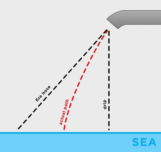
Figure 8. The diagram shows the two limits on the path that oil can take as it falls downward to the sea.
261 To perform his initial calculations, Professor Wereley used two photographs taken on 21 August 2009 (designated as PTT.617.003.9947 and PTT.617.003.9939); one photograph taken on 22 August 2009 (designated as PTT.620.003.8765); one photograph taken on 26 August 2009 (designated as PTT.600.026.5696); one photograph taken on 9 September 2009 (designated as PTT.620.003.8819); and one photograph taken on 3 November 2009 (designated as PTT.620.004.0916). Thus, the oil flow from the horizontal drain pipe was measured on five days. Eight separate measurements were made. Professor Wereley summarised the results of his analysis and calculations in a table (Table 2):
Table 2. Summary of measurements | ||
Date | Image Name | Oil Flow Rate (Bbl/day) |
21 August 2009 | PTT.617.003.9947 | 1250 |
21 August 2009 | PTT.617.003.9947 | 362 |
21 August 2009 | PTT.617.003.9939 | 1582 |
21 August 2009 | PTT.617.003.9939 | 668 |
22 August 2009 | PTT.620.003.8765 | 417 |
26 August 2009 | PTT.600.026.5696 | 1170 |
9 September 2009 | PTT.620.003.8819 | 715 |
3 November 2009 | PTT.620.004.0916 | 464 |
262 Professor Wereley calculated the cumulative volume of oil spilled as follows:
17.2 Given the quantitative measurements and the qualitative observations, it seems clear that the oil continued flowing throughout the course of the oil spill. Based on the materials which I have been asked to consider, I am unable to observe any quantitative trend regarding the oil volume flow rate. For example, the volume flow rate of the oil exiting the horizontal drain pipe measured on 9 September 2009, was both considerably higher and lower than measurements for volume flow rates in August 2009. Consequently, it is my opinion that the best way to estimate the oil flow rate over the course of the spill is to average the first seven numbers in Table 2. These seven measurements are representative of the oil volume flow rate before the well head platform caught fire. I have excluded the measurement for 3 November 2009 as it is only representative of the short period of time that the well head platform was on fire. It is clear that less oil was spilled into the ocean when the well head platform was on fire as much of the oil burned and did not drain into the sea. The best estimate of the oil volume flow rate between 21 August 2009 and 31 October 2009 is:
Qavg = (1250+362+1582+668+417+1170+715)/7 = 881 bbl/day
17.3 The total volume of oil spilled is then the sum of the average daily oil volume flow rate times the number of days before the well head platform caught fire and the oil volume flow rate after the well head platform caught fire times the number of days before the well was killed:
Total volume = 72 days x 881 bbl/day + 3 days x 464 bbl/day = 64,824 bbl
(Emphasis in original.)
Criticism of Professor Wereley’s analysis and calculations
263 The respondent called Dr Zaldivar to prepare a report responding to Professor Wereley’s first report. In his report, Dr Zaldivar said that there were many errors, assumptions and simplifications in the methodology that Professor Wereley had used to calculate flow rate. He identified four matters which he saw as “key deficiencies” which, in his opinion, rendered Professor Wereley’s conclusions “completely unreliable and invalid”.
264 First, Dr Zaldivar said that Professor Wereley’s treatment of the effect of wind on the oil draining from the horizontal drain pipe was incorrect because Professor Wereley did not correctly account for the horizontal and vertical components of wind drag on fluid velocity. Dr Zaldivar argued that, when the correct equations are taken into consideration, it is not possible to calculate a flow rate using Professor Wereley’s approach. This is because there were too many unknown variables. Dr Zaldivar argued that, because the formulation used by Professor Wereley was incorrect, all the calculated flow rate results should be “considered unreliable and invalid”. Dr Zaldivar also pointed out that Professor Wereley had adopted inconsistent assumptions: Professor Wereley had argued that wind friction could be ignored but, in his calculations, he had added a horizontal component of wind speed to the fluid velocity where the fluid exits the horizontal drain pipe.
265 Secondly, Dr Zaldivar identified a unit conversion error which, he said, caused Professor Wereley’s calculations to be “fundamentally flawed”. Dr Zaldivar contended that, when this error was corrected, the results of Professor Wereley’s calculations were “completely out of the range of reality” and “nonsensical”. Dr Zaldivar argued that this underscored (what he saw as) the “fundamental unreliability” of Professor Wereley’s method.
266 Thirdly, Dr Zaldivar said that Professor Wereley had incorrectly assumed that the flow exited the horizontal drain pipe at a 45° angle (the exit angle of the pipe bend at the distal end of the drain pipe). In Dr Zaldivar’s opinion, the length of the pipe bend was not sufficiently long to cause the entire flow to deviate along the bend, especially at higher velocities. Dr Zaldivar replicated Professor Wereley’s calculations but changed the exit angle to 30°. This showed that Professor Wereley’s fluid velocity was nearly 86% greater for an exit angle that was only 50% greater than the angle which Dr Zaldivar used. According to Dr Zaldivar, this demonstrated the sensitivity of Professor Wereley’s calculations to the exit angle selected.
267 Fourthly, Dr Zaldivar said that Professor Wereley’s fraction filled calculation (i.e., how much of the pipe was filled with oil) was incorrect due to several factors, namely:
(a) Professor Wereley had treated the fraction filled as 100% in cases where, in Dr Zaldivar’s view, there was insufficient photographic information available to make that determination (Dr Zaldivar said that Professor Wereley’s method of estimating the apparent fraction filled was “just a guess”);
(b) the photographs that Professor Wereley had used showed only the “apparent fraction filled” (meaning that, as fluid exiting the drain pipe does not have enough time to bend completely along the pipe bend, the apparent fraction filled as seen at the exit of the pipe bend will always be higher than the actual fraction filled in the horizontal portion of the pipe: in other words, there is an appearance that the pipe is fully filled when, in fact, it is not); and
(c) Professor Wereley had assumed that there was no water and no entrained gas in the liquid phase; any water would reduce the calculated volume of the oil that was discharged and entrained gas flowing in or with the oil would reduce the oil flow rate.
268 Dr Zaldivar advanced a number of other criticisms. He criticised Professor Wereley’s use of three of the photographs to carry out his calculations. In essence, Dr Zaldivar argued that the photographs were unsuitable, in various ways (including their low resolution), for the way in which Professor Wereley used them. With respect to two of the other photographs, Dr Zaldivar criticised the way in which Professor Wereley used them.
269 Dr Zaldivar criticised Professor Wereley’s analysis and calculations. In particular, he criticised the way in which Professor Wereley arrived at his calculation of cumulative volume. Dr Zaldivar argued that there was a clear trend of decreasing flow rate over time. He said that Professor Wereley’s estimated cumulative volume of oil discharged (64,824 bbl) was “between three and four times too high just based on the way [Professor Wereley] performs the cumulative calculation”.
270 Dr Zaldivar also argued that Professor Wereley had used an incorrect measurement for the internal diameter of the horizontal drain pipe (Professor Wereley used its nominal measurement of 8” whereas Dr Zaldivar said the internal diameter of the pipe was 7.813”). Dr Zaldivar said that Professor Wereley’s incorrect pipe diameter accounted for an over-estimate of the calculated flow rates by 4.6%.
271 Dr Zaldivar also argued that Professor Wereley’s analysis of the photographs had not accounted for perspective effects due to the wind velocity.
272 Further, Dr Zaldivar argued that Professor Wereley had failed to determine the uncertainty of the estimates he had used in performing his calculations. Dr Zaldivar said that if Professor Wereley had performed a scientific analysis of the uncertainty in this approach, he would have found that some of the inputs he used greatly affected the flow rates calculated using his methodology.
273 Dr Zaldivar also introduced the possible confounding effect of the activation of the fire systems on the platform and drilling rig at the time of the spill. He argued that if the fire systems were active, then water from those systems would have mixed with oil in the horizontal drain. If so, Professor Wereley would have overstated the observed flow from the horizontal drain because that flow would have included a potentially large amount of seawater.
274 It is convenient at this point to record that there is no direct evidence before me that the fire systems had, in fact, been activated at the time the photographs were taken. It is only Dr Zaldivar’s speculation that such systems might have been activated. He sought to give life to this speculation by referring to one photograph showing a difference in the colour of the flow from the vertical drain pipe on the West Atlas rig (a lighter colour) compared to the flow from the horizontal drain pipe on the wellhead platform (a darker colour). I am not prepared to draw any conclusion from this colour difference. It is very indirect evidence and, on the other evidence before me, the colour difference could be attributable to any one or more of a number of different factors. I am not satisfied on the evidence that the fire suppression systems had been activated in the photographs on which Professor Wereley relied. I would add that, had the fire suppression systems been activated, then there seems to have been no reason why the respondent could not have called direct evidence of that very matter.
275 Dr Zaldivar expressed his overall conclusions as follows:
5.1 Dr. Wereley used a method of estimating fluid velocity by applying a mathematical formulation that describes the trajectory of the fluid exiting the drain pipe and calculating a fluid velocity that predicted a trajectory that matches the observed trajectory in photographic evidence. In the process, he overly simplified or made unjustified assumptions about several factors:
1) He assumed that the exit angle would always be 45° downward to the horizontal, which is incorrect based on the short length of pipe bend at the end of the horizontal drain pipe.
2) He assumed that the apparent fraction filled in the photographs is the fraction filled in the horizontal pipe without regard for the fact that fluid at the edge of the horizontal pipe had to travel a mere 11.2 inches before it struck the top surface of the pipe bend, which would result in an apparent fraction filled of 100%. He also ignores the perspective effects on apparent fraction filled.
3) He simultaneously assumed that air offers both zero resistance by ignoring the effect of air in calculating the trajectory, and infinite resistance by adding the horizontal component of wind velocity to the fluid exit velocity immediately upon its exit. He also assumed that wind velocity had no vertical component, and that the off-plane component of wind velocity had no apparent effect on the observed trajectory.
4) He assumed that there is no water in the fluid exiting the horizontal drain pipe while providing no scientific basis for his assumption.
5) He assumed that there is no gas entrainment in the liquid, while multiphase correlations show that at high liquid velocities, gas would certainly be entrained as dispersed bubbles in the liquid phase. He makes no effort to address this on a scientific basis.
6) His calculation of cumulative volume discharged heavily weights the flow rates during the first five days of the spill.
7) He made several mistakes in his report and did not consistently report all the calculated parameters, e.g., wind velocity is only reported in the first calculation and completely ignored in the rest of the calculations.
8) He made no effort to extrapolate and compare the trajectory, which is calculated based on very few points near the exit of the drain pipe, to the longer trajectories visible in the photographs.
5.2 Beyond these mistakes and deficiencies in the report, the most important mistake is his conversion factor from ft3/s to bbl/d. Fixing this mistake puts his results in a range of flow rates that are wildly inconsistent, by an order of magnitude, with the reservoir simulations that were used in support of the well kill effort. The fact that the well kill effort was successfully performed lends credence to the reservoir simulations, based on which the oil flow potential of the well was estimated to be around 1500 bbl/d.
5.3 Based on all these factors, my opinion is that Dr. Wereley’s report cannot be relied upon to obtain a scientifically sound estimate of the total volume discharged during the incident. Even in the event one decides to accept his methodology to calculate flowrate, I found several omissions and mistakes that resulted in an overstatement of the calculated flowrates.
276 Professor Wereley took on board Dr Zaldivar’s criticisms. He prepared a second report.
277 Professor Wereley accepted that there was inconsistency in assuming that the friction of the oil with the surrounding air was unimportant while at the same time assuming that the oil jet assumed the speed of the wind surrounding it. Professor Wereley accepted that the inconsistency needed to be resolved. He held to the assumption that the oil jet is not slowed considerably by the air because, at the exit of the horizontal drain pipe, the air only had a short time to act on the jet. However, Professor Wereley removed from his calculations the assumption that the oil immediately matched the speed of the air around it. In other words, he proceeded on the basis that the oil stream does not respond to the air drag near the horizontal drainpipe exit. As Professor Wereley put it, this approach is equivalent to saying that the momentum of the oil jet is large compared to the drag acting on it near the pipe exit. Professor Wereley said that this was a conservative assumption because neglecting the effect of drag on the jet (however small) would lead to a smaller jet speed in his calculations.
278 Professor Wereley accepted that he had made a unit conversion error in his calculations.
279 Professor Wereley accepted that the flow rate is dependent on the angle of the oil jet as it leaves the horizontal drain pipe. He therefore modified his jet flow calculations by extracting the exit angle from a “best fit” model of the jet motion, rather than assuming it from the geometry of the horizontal drain pipe.
280 With respect to the calculation of the fraction filled, Professor Wereley rejected the criticism that his methodology was “just a guess”. He said that his analysis of the photographs was based on commonly used methodologies in the open channel flow field (the study of flows in partially filled conduits, pipes and the like). As to Dr Zaldivar’s criticism that there was insufficient spatial resolution to see the jet height, Professor Wereley used a method to determine the fraction filled which involved deriving size ratios of the height of the jet exiting the horizontal drain pipe in images with better resolution, where the jet can be seen exiting the pipe and flowing at a more or less steady flow rate as it drops to the sea, and applying those ratios to the affected, lower resolution images.
281 Professor Wereley maintained his view that there was an insignificant amount of water in the discharge. Nevertheless, to compensate for uncertainties, he calculated what the flow rate would be if the flow contained 10% water. The figure of 10% appears to be based on a statement in the respondent’s Dynamic Kill Simulations and Evaluations report (relied on by the respondent to calculate the parameters for the operation to “kill” the well in order to stop the spill) that said that the condensate contained “less than 10% water cut”.
282 Professor Wereley agreed that air could be mixed with the oil in the drain system in such a way that the two would not separate as quickly as he had originally assumed. However, he considered that Dr Zaldivar had over-predicted the proportion of gas that might be entrained. Professor Wereley accepted that the flow out of the horizontal drain pipe is pulsatile. It was sometimes fast, and sometimes slow, which supported the view that the oil was mixed with air. As I have noted, the drain system is comprised of numerous straight sections of pipe with many 90° elbows and other fittings along its path. Professor Wereley explained that at each of these elbows or other fittings, the turbulent flow in the drain system thoroughly mixes the air carried along by the oil flow with the oil itself. Many small bubbles would be generated by repeated agitation, creating a mixture that would not be quickly separated. As a result, Professor Wereley modified his jet flow calculation by assuming that the liquid flowing out of the horizontal drain pipe is carrying air bubbles mixed in it.
283 With respect to Dr Zaldivar’s contention that, in calculating cumulative volume, Professor Wereley should have adopted a model in which oil flows slow with time, Professor Wereley observed that, while that may be the normal behaviour of an oil well, the H1 Well was not performing normally. He suggested, for example, that it was possible that the hole in the cement shoe would have eroded over time such as to cause an increase in flow. He said that, in order to make a “fact and observation-based measurement”, he had only used the data that he, himself, could measure. He did not use an outside model of the expected reservoir behaviour. However, as each instantaneous spill flow rate measurement was representative of the spill on a different date, and those dates were arbitrarily spaced through the duration of the spill, Professor Wereley re-calculated the spill volume using a method common in engineering called the trapezoidal rule, rather than relying on a simple average of all measurements he made. As Professor Wereley explained it, by applying the trapezoidal rule, instantaneous flow measurements (bbl/day) are turned into a total spill volume (bbl).
284 Professor Wereley recognised that there was uncertainty in each of the main components of his measurements, including: the scale factor; the speed of the flow calculation; the fraction filled calculation; the volume fraction of gas carried by the flow; and the fraction of the condensate that is water. He reasoned that the uncertainties in the scale factor and flow speed calculations could be ignored in the presence of the much larger uncertainties in other quantities.
285 In relation to the possible activation of the fire systems, Professor Wereley noted that one of the assumptions with which he had been provided was that all electricity to the West Atlas rig was turned off by 9.00 pm on Friday, 21 August 2009. If so, any fire suppression systems that may have been operating would have ceased by that time and any fire suppression fluids would have ceased running off the rig at that time or shortly thereafter. Two flow measurements that Professor Wereley calculated were based on photographs taken on 21 August 2009 during the day. He acknowledged that, consequently, it is possible that some part of the calculated flow was water from the fire suppression system on that day. However, as I have said, I am not satisfied on the evidence that the fire suppression systems had been activated in the photographs on which Professor Wereley relied.
286 Professor Wereley then re-computed his flow rate calculations and presented his revised results in his second report as follows:
15.1 My calculations have been revised incorporating the following factors that were discussed in detail above:
(a) The correct inner pipe diameter of 7.813 inches.
(b) The drag of the surrounding air on the jet just after it leaves the HDP is neglected.
(c) The units are properly converted from ft3/sec to bbl/day.
(d) The downward angle of the oil jet emerging from the HDP is extracted from the jet trajectory rather than imposing a 45 degree angle.
(e) Fraction filled is treated differently in cases where the spatial resolution of the photo is too low to directly and accurately judge the fraction filled (i.e. PTT.600.026.5696) or cases where there is a fast and slow flow in the same photo and only one of those is emerging from the HDP exit in the photo (PTT.617.003.9947 and PTT.617.003.9939).
(f) The model accounting for the air mixed in and carried along with the oil flow as bubbles using Gomez’s (2000) equation.
(g) The calculation of total spill volume has been made by integrating the measurements made using the trapezoidal rule.
15.2 In order to calculate the total amount of oil spilled into the environment, the instantaneous oil spill rates (i.e. bbl/day) must be integrated into a single number. In order to bound the maximum and minimum possible spill sizes, the uncertainties in the fraction filled, volume fraction of gases, and water content have been considered as shown in Table 2 below.
Table 2. Oil Spill Flow Rates | |||||
Date | Image Name | Day # | Exp Oil Flow Rate (bbl/day) | Max Oil Flow Rate (bbl/day) | Min Oil Flow Rate (bbl/day) |
21 Aug | PPT.617.003.9947 | 1 | 19100 | 21000 | 13300 |
0 | 0 | 0 | |||
21 Aug | PPT.617.003.9939 | 1 | 18900 | 20800 | 13200 |
9400 | 10300 | 6500 | |||
22 Aug | PPT.620.003.8765 | 2 | 8300 | 9100 | 5800 |
26 Aug | PPT.600.026.5696 | 6 | 10500 | 11600 | 7300 |
9 Sept | PPT.620.003.8819 | 20 | 12300 | 13500 | 8600 |
3 Nov | PPT.620.004.0916 | 75 | 3600 | 4000 | 2500 |
287 After applying the trapezoidal rule, Professor Wereley calculated that the total oil spill volume over the period of the spill was between 452,000 and 714,000 bbl. This is approximately 6,000 to 9,000 bbl/day.
288 The presentation of Professor Wereley’s revised calculations did not end the disagreements between the two experts on this question or bring them any closer. In fact, the area of disagreement was widened by some of the accommodations that Professor Wereley had made to meet Dr Zaldivar’s criticisms. For example, a new area of disagreement was the way in which Professor Wereley had analysed and digitised the trajectory of the oil jet from the horizontal drain pipe in his second report.
289 The various disagreements carried on into a Joint Report prepared by the four experts on spill volume (the Joint Report on Volume), and into the concurrent evidence session. Dr Zaldivar maintained that, notwithstanding the revisions which Professor Wereley made to accommodate his (Dr Zaldivar’s) criticisms, there were many errors, assumptions and simplifications in Professor Wereley’s methodology that rendered his conclusions “completely unreliable and invalid”. He also argued that the uncertainties associated with the inputs that Professor Wereley used, and their impact on the uncertainty of the calculated flow rate, had been “grossly understated” by Professor Wereley and provided “false confidence in the validity of the total volume estimate”.
290 No further light will be thrown on the differences between Professor Wereley and Dr Zaldivar by further summarising that debate in these reasons. The following matters are, however, important.
291 First, Dr Zaldivar’s instructions from the respondent were to prepare a report responding to Professor Wereley’s first report. Dr Zaldivar steadfastly interpreted these instructions as meaning that he was not to provide an estimate of spill volume and that he was confined to critiquing Professor Wereley’s methodology and calculations. Indeed, in the Joint Report on Volume he specifically identified this as his role. It was a role he performed with some vigour.
292 Secondly, Professor Wereley’s task was to find the best method possible, in the circumstances of the available evidence (which, admittedly, was limited), to calculate spill volume. As Professor Wereley himself explained, there is no “ground truth” in his calculations. Rather, they stand as one analysis through which the Court can gain an appreciation of the likely size of the spill (in terms of volume and rate of discharge) from objective evidence rather than unsupported assertion. Three experts provided that assistance in terms of using their expertise to arrive at reasoned calculations. Dr Zaldivar did not. His role was a more limited and directed one. Even then, the main thrust of his criticisms was to raise the prospect of error, without demonstrating that there was error, or error that would lead to an appreciably different outcome in actual result. Thus, his contentions that Professor Wereley’s calculations were “unreliable” or “invalid” reside in, and do not transcend, the realm of argument and debate.
293 The notable exceptions to this were Dr Zaldivar’s identification of Professor Wereley’s conversion error and Professor Wereley’s inconsistent inclusion of a wind drag factor in the equations he used. However, when these errors were pointed out, Professor Wereley quite properly accepted them as such, and made corrections to accommodate for them. Dr Zaldivar did perform a calculation—based on what he regarded to be Professor Wereley’s flawed methodology—in which he integrated the area under the curve to obtain a cumulative discharge volume. By this calculation, Dr Zaldivar arrived at a total volume spill of 16,178 to 21,181 bbl. However, in keeping with the limitations he placed on the instructions he had been given, Dr Zaldivar did not undertake his own analysis of the volume of oil spilled, or provide his own calculations based on that analysis. Thus, Dr Zaldivar did not present an alternative estimate of the amount of the oil spilled which could be exposed to evaluation and comment by his fellow experts—in particular, which could be set against Professor Wereley’s analysis.
294 In this regard, Dr Zaldivar did present several alternative analysis options in the Joint Report on Volume. But, having done that, he once again retreated to the position that he had received no instructions to proceed with them. He said that he would “undertake any of these options … upon receiving written instruction from the Court and an agreement that resolves how I will be compensated for such efforts”.
295 I do not regard it to be the role of the Court in an adversarial trial system to give such instructions or provide advice to parties as to the evidence they should adduce. In the end, Dr Zaldivar’s discussion of these options provided no meaningful assistance to the Court. The applicant submitted, with considerable justification, that Dr Zaldivar’s contribution to the topic of the volume of oil spilled could best be described as that of a “sniper” firing shots at Professor Wereley’s work: see the analogy described by Martin J in Mineralogy Pty Ltd v Sino Iron Pty Ltd (No 16) [2017] WASC 340 at [741] – [743].
296 Thirdly, the thrust of Dr Zaldivar’s various criticisms of Professor Wereley’s work seems to be that it was carried out incompetently, both methodologically and as a matter of computation or calculation. If that is what Dr Zaldivar intended to convey, then that is certainly not my impression of Professor Wereley as an expert, or of his evidence. There was no challenge to Professor Wereley’s expertise.
297 Professor Towler, who calculated oil volume using material balance (see below), reviewed the reports prepared by Professor Wereley and Dr Zaldivar and expressed the opinion that the methodology that Professor Wereley had used to determine flow rate was, in fact, correct. For completeness, I record that Professor Blunt, the other expert on oil spill volume, did not comment on Professor Wereley’s work or Dr Zaldivar’s criticisms.
298 Whilst there were difficulties in carrying out a flow rate analysis on the evidence available to Professor Wereley, and whilst the possible impact of those difficulties on the estimates provided by Professor Wereley must be recognised, I do not accept that his estimates can simply be cast aside and ignored as “unreliable” or “invalid”.
299 Fourthly, Professor Towler expressed the opinion that the original estimate of spill volume made by Professor Wereley (i.e., in his first report) was the most reliable estimate using the flow rate method. He noted that, when Professor Wereley’s conversion error was corrected, the total volume of oil spilled would be in the order of 3.64 million bbl. He said that the averaging used by Professor Wereley in his first report was likely to be more accurate than applying the trapezoidal rule, because reservoir flow rates tend not to decline much in the first 75 days of production. In fact, a typical decline rate for a petroleum reservoir is about 10% per annum. This would amount to a decline of about 2% over 75 days. Therefore, according to Professor Towler, Professor Wereley’s original assumption of a constant rate for 72 days was reasonable.
300 Relatedly, Professor Towler disagreed with Dr Zaldivar’s suggested method of integrating the measured flow rates into a total spill volume, which was based on a decline rate of 85% over 75 days. Professor Towler said that this decline rate was quite unrealistic and led to a decreased estimate of the total volume spilled.
301 Professor Towler also pointed out that when Dr Zaldivar carried out his calculation of the amount of oil spilled using Professor Wereley’s methodology, he (Dr Zaldivar) committed the same conversion error for which he had criticised Professor Wereley. Professor Towler’s evidence was that if Dr Zaldivar had used the correct unit conversion factor in his calculations (i.e., the one Dr Zaldivar said that Professor Wereley should have used), his total spill volume would have been between 906,000 and 1.18 million bbl, not 16,178 to 21,181 bbl.
302 Fifthly, Professor Towler noted that the H1 Well was designed to be able to flow at 28,500 bbl/day, through a tubing string of 5.5” (external diameter). However, this tubing string had not been installed before the blowout. Consequently, the reservoir fluid was free to flow through the 9 5/8” casing. This means that the oil would have been able to flow at more than 28,500 bbl/day. On the evidence, there was also an expectation that, once completed, the well would flow at 9,000 to 10,000 bbl/day, under controlled conditions. However, during the blowout, the conditions were not controlled and, according to Professor Towler, it would be expected that the well was flowing at a rate that was not restricted by its well potential.
303 Sixthly, as I have already noted, Professor Wereley’s calculations were based only on the flow from the horizontal drain pipe and not the other sources of oil flow which would have contributed to the volume of oil spilled into the sea over the 75 day period that the well was uncontrolled.
304 Material balance is an independent method of verifying the amount of oil that was lost from the reservoir feeding the H1 Well during the blowout. To conduct the analysis, the pressure loss in the reservoir is used. Utilising the known volumes of oil and gas originally in the reservoir, the original and final pressures before and after the blowout, the properties of the reservoir fluid, and an estimate of the water that has invaded the reservoir from the aquifer during the blowout, it is possible to calculate the fluid lost from the reservoir.
305 Professor Blunt described the material balance method in the following simplified terms:
3.4 ... When the well is drilled through the reservoir, it encounters the fluids in the reservoir rock: oil, natural gas and water. These fluids are stored at very high pressures in tiny pore spaces. The rock is under enormous pressure from the weight of rock above it. The well allows a release of oil out of the reservoir to the surface. As oil, water and gas start to flow through the rock’s connected pores, the pressure of the oil in the reservoir decreases. When the pressure decreases, the remaining oil expands, pushing the oil out of the reservoir. As the pressure of the fluids within the rock pores drops, the rock is compressed down, squeezing the pore spaces, pushing out more oil. The material balance principle says that the volume of oil, gas and water that comes out of the reservoir must be equal to the combined volume expansion of oil, water and gas, and the compression of the rock pore space. To calculate the oil produced from this fluid expansion and rock compression, only the compressibility of the fluids and rock, the size of the reservoir connected to the well, and the change in pressure need to be determined. These are the three variables that will be discussed throughout the remainder of this report.
3.5 In even simpler terms: the pressure-driven change in the volume of oil, gas, water and rock pore space in the reservoir is equal to what comes out of the well. This is the central concept in reservoir engineering: to relate what was produced to changes in the reservoir. We keep track of the volume of oil produced by calculating the volume of oil displaced from fluid expansion and pore contraction.
3.6 The advantage of the material balance approach is that it does not require knowledge of changing flow rates over time, or other indirect measures of volume, such as the extent of the spill, instead computing directly the total amount of oil produced.
306 Using the material balance method, Professor Towler determined that the amount of oil spilled during the blowout was in the range of approximately 520,000 bbl to 3 million bbl, with the most likely amount to be about 1.8 million bbl (on a simple average, 24,000 bbl/day). Professor Blunt determined that the amount was between 57,000 bbl to 74,000 bbl, with a mid-range value of 69,000 bbl (on a simple average, 920 bbl/day). He nevertheless accepted in cross-examination that, within the range of uncertainty, the volume of oil released, by reference to his calculation, could have been 100,000 bbl or more (on a simple average, approximately 1,333 bbl/day).
307 There is, obviously, a significant difference between the two ranges that were calculated. The significant difference between them is the approximations that each had made.
308 To explain, the Montara oil field has a gas cap above the oil. It is also connected to a large body of underground water (aquifers). The water in the aquifers, and the gas in the cap, expanded when the pressure dropped during the blowout.
309 Professor Blunt assumed, for the purposes of his calculation, that the expansion of the water was matched by the production of water, and that the expansion of gas was matched by gas production. Therefore, on his approach, the oil produced and spilled equalled the expansion of oil.
310 Professor Towler considered Professor Blunt’s material balance model to be highly simplified. He argued that Professor Blunt had ignored several important drive mechanisms. According to Professor Towler, the most important of these was the invasion of water from the aquifer into the hydrocarbon reservoir. As water invades the reservoir, it pushes oil in front of it and drives the oil towards the producing well. Consequently, oil is preferentially produced over water. Professor Towler saw the aquifer influx as the primary drive mechanism, with gas expansion and oil expansion as the secondary and tertiary drive mechanisms, respectively. The three mechanisms were accounted for in his model, whereas Professor Blunt’s simplified model relied on oil expansion alone for estimating the volume of oil spilled.
311 Professor Towler said that there were three aquifers contributing to a strong water drive. The first is an aquifer directly connected to the Montara hydrocarbon reservoir, which feeds the H1, H2, and H3 Wells. Professor Towler opined that this aquifer was the main contributor to the aquifer influx during the blowout. It contained 6.5 billion bbl of water, had a reported permeability of 2000 milli-darcies (mD) (a very high permeability) and a thickness of 44 m. The second aquifer, referred to as the Regional Aquifer, contained 24 billion bbl of water and was also connected to the Montara hydrocarbon reservoir. The third aquifer was located in the region of a formation called the Plover Formation. It contained 400 billion bbl of water. Professor Towler estimated that approximately 3.6 million bbl of water invaded the Montara hydrocarbon reservoir during the blowout. This was a very small fraction (0.0066%) of the 6.5 billion bbl of the water in the first aquifer, and an even smaller fraction of the water in the other two aquifers.
312 Professor Blunt considered Professor Towler’s estimate of water influx to be excessive. In his view, the water flow would have been impeded by faults in the reservoir and aquifer, and that these impediments had to be accounted for in the calculation. In assessing the degree of impediment, Professor Blunt relied on aquifer properties analysed in a study called the Montara Aquifer Study (2003) (the Montara Aquifer Study). Professor Blunt estimated the aquifer influx to be 57,000 bbl of water. This was based on the assumed permeability used in the Montara Aquifer Study of the connection between the Plover Formation and the Montara hydrocarbon reservoir, recorded as 33 mD. He argued that if the aquifer influx had been of the order estimated by Professor Towler, the spill would have been comprised almost entirely of water.
313 Whilst not disputing that account had to be taken of the tortuosity between the large aquifer in the Plover Formation and the oil and gas accumulation in the Montara hydrocarbon reservoir, Professor Towler argued that, in using the figure of 33 mD, Professor Blunt had used the wrong value for permeability because, during the blowout, the aquifer that was invading the reservoir was the 6.5 billion bbl in the immediate vicinity. In other words, there was no basis to assume that the permeability of this aquifer was the same as the permeability of the more distant aquifer in the region of the Plover Formation. Therefore, in his analysis, Professor Towler used an aquifer permeability of 1000 mD, even though the Montara Aquifer Study reported the permeability of the first aquifer as 2000 mD. In his oral evidence, Professor Towler said that he selected the figure of 1000 mD in order to be conservative. He also assumed that, in relation to this aquifer, the faults had minimal effect.
314 A further matter pointed out by Professor Towler was that, even though Professor Blunt estimated the aquifer influx to be only 57,000 bbl of water, this figure was not taken up by Professor Blunt; aquifer influx did not appear in his material balance equation.
315 In the Joint Report on Volume, Professor Towler and Professor Blunt agreed that determining the amount of water influx during the blowout represented a significant uncertainty. They agreed that the well bore was sufficiently conductive to allow a release of more than 1 million bbl of oil if the flow were unimpeded. As I have said, the issue on which they disagreed was how significantly the oil flow would be impeded. The evidence does not enable that determination to be made. I am left only with the separate possibilities posited by Professor Towler and Professor Blunt.
316 On the evidence before me, I am satisfied that the oil released over the 75 days of the spill was far greater than the suggested rate of 200 to 400 bbl/day. Of course, one will never know with certainty the volume of oil actually spilled in that period or the rate at which it was released. But taking the lowest volume estimate in the evidence adduced in this proceeding (Professor Blunt’s mid-range estimate), and assuming a relatively steady rate of release over the period (a simplifying assumption I consider to be reasonable for my purposes), it can be seen that, as a minimum, the oil would have been released at a rate of 920 bbl/day. This is significantly greater than the rate assumed in Dr French-McCay’s base case modelling (400 bbl/day).
317 The applicant submitted that once it is accepted that the rate of release was greater than 200 to 400 bbl/day, the precise volume of oil spilled need not be quantified. That might be so. However, I should record that I am satisfied that it is likely that the volume of oil spilled was far greater than Professor Blunt’s estimate and that, correspondingly, the oil was spilled at a far greater rate than implied by that estimate. Professor Blunt and Professor Towler acknowledged that there is considerable uncertainty involved in the volume of the aquifer influx that would drive the release of oil. This uncertainty is reflected in the two estimates made on the basis of a material balance calculation. I note, however, their agreement that the well bore was sufficiently conductive to allow a release of more than 1 million bbl of oil (on a simple average, approximately 13,333 bbl/day over the period in question) if the flow were unimpeded.
318 Between Professor Blunt’s and Professor Towler’s respective estimates is the estimate made by Professor Wereley in his second report (6,000 to 9,000 bbl/day). The estimate made in Professor Wereley’s first report significantly exceeds this rate (once his conversion error is corrected).
319 I accept that there are difficulties (and hence uncertainties) in making a flow rate calculation on the basis of the available evidence. But even taking his lower estimate, it should be recognised that Professor Wereley’s analysis was directed to a single source of discharge (the horizontal discharge pipe on the wellhead platform), and not the other sources of discharge at the H1 Well.
320 Taking all the evidence on spill volume into account, I am satisfied on the balance of probabilities that, over the period in question, oil was being discharged at an uncontrolled rate in excess of the ranges considered in Dr Hubbert’s modelling (in other words, in excess of 2,500 bbl/day).
321 It is appropriate to recall that the modelling carried out by the respondent in 2011 and revisited in 2013 included a “loss of well control” spill over 77 days, discharging 84,966 m3 or 534,380 bbl of Montara oil at rates varying between 3,802 m3/day or 23,912 bbl/day down to 690 m3/day or 4,341 bbl/day. This scenario was regarded as credible.
322 Dispersants were applied to the oil spilled from the H1 Well in the period 23 August to 1 November 2009.
323 The term “dispersant” is used to refer to a variety of chemical spill-treating agents that promote the formation of small droplets of oil which then “disperse” throughout the top layer of the water column.
324 Dispersants are mixtures of two components: surfactants and solvents. Surfactants (surface-active agents) are the active ingredients of dispersants which are mixed with a solvent. The solvent has two functions: it reduces the viscosity of the surfactant, which enables it to be sprayed, and it promotes the penetration of the surfactant into the oil slick. The surfactants in dispersants are also used in many common household products, including soaps, skin creams, baby bath, cosmetics, shampoos, mouthwash, intestinal medications, and even food.
325 Some portion of released oil will disperse into the water column whether or not chemical dispersants are used. Natural dispersion of floating oil is a process facilitated by wave action that breaks the oil into small droplets. It is affected by the properties of the oil and the amount of wave energy at the sea surface. In general, oils with lower viscosity are more amenable to natural dispersion than those with higher viscosity. Likewise, higher wave energy produces more natural dispersion.
326 Dispersants work because surfactant molecules have two distinct and linked parts: one is lipophilic (attracted to oil) which orients itself into the oil; the other is hydrophilic (attracted to water) which orients itself into the water. The surfactant molecules align themselves at the oil/water interface and reduce interfacial tension. Interfacial tension causes oil molecules to stick to each other in the form of a slick. High interfacial tension keeps the slick intact on the surface. The surfactant molecules interfere with this tension by reducing forces between the oil molecules, which enhances the breakup of an oil slick. When mixing energy is applied (for example, through wind, waves, and currents), the dispersant-treated oil slick will break up into many tiny microdroplets that are less than 100 µm in diameter. The microdroplets generally tend to stay suspended in the water column, while larger droplets are more likely to float back to the surface and re-coalesce into the slick.
327 One motivation for using dispersants is to treat an oil slick in the hope that the surface slick does not contact a shoreline. A second motivation is to reduce the impact of the oil on birds and mammals on the water surface. A third motivation is to promote the biodegradation of oil in the water column.
328 There is some dispute in the evidence as to whether biodegradation is enhanced. Dr Fingas said that the effect of dispersants on biodegradation is still a matter of dispute and that some current dispersant formulations can, in fact, inhibit biodegradation. He said that no enhancement of biodegradation is clearly shown in any recent studies.
329 Dr Coelho strenuously disputed Dr Fingas’ statements in this regard, noting that Dr Fingas had cited no references in support. She said that Dr Fingas’ statements were contrary to dozens of peer-reviewed publications on dispersed oil degradation, which she referred to and summarised in her first report. Dr Coelho said that the use of dispersants provides naturally-occurring, oil-degrading bacteria greater access to the oil by creating a diluted mixture of small oil microdroplets. The microdroplets are inherently more biodegradable than large, un-treated oil droplets because a greater surface area-to-volume ratio is available for microbial attack.
330 There was also disagreement between Dr Fingas and Dr Coelho about the effectiveness of dispersants both generally and in relation to their application to the oil spilled from the H1 Well.
331 Dr Fingas said that the main cause of dispersant ineffectiveness is high oil viscosity, which results in little dispersant mixing of the oil. He said that when dispersant droplets hit viscous oils they may run off into the water column rather than mix with the oil.
332 Dr Fingas said that the second cause of ineffectiveness is the lack of stability of the oil droplets in the water column over time. He referred to the phenomenon of resurfacing oil, which is the result of two separate processes: destabilisation of the oil-in-water emulsion and desorption of surfactant from the oil-water interface. The latter results in less surfactants in the oil droplets, and thus more coalescence of the droplets. The more coalescence that occurs, the larger the droplets will be, and the faster they will rise to the surface, reforming a slick.
333 In response, Dr Coelho referred to certain literature dealing with the effectiveness of dispersants on viscous oils. She also referred to multiple field studies on dispersant effectiveness which, she said, have repeatedly documented the fact that once a dispersant is applied, the dispersed oil microdroplets mix into the underlying several metres of water column. She said these microdroplets are diluted horizontally and vertically into the ocean so that the individual microdroplets cannot collide with each other. If they cannot collide, they cannot re-coalesce. In this connection, Dr Coelho drew a distinction between closed and open systems. The ocean is an open system in which the dispersed oil droplets dilute such that the tendency for them to coalesce is minimised. Dr Coelho said that this is a critical fact that inhibits suspended, neutrally-buoyant microdroplets from reforming into larger, positively-buoyant drops that rise to the surface and again become a surface slick.
334 With regard to the application of dispersants applied to the oil spilled from the H1 Well, Dr Fingas referred to data obtained from reports prepared by Leeder Consulting of the concentrations of oil under the oil plumes treated with dispersants at the time of the spill. These were so-called “grab samples” from which Leeder Consulting measured total petroleum hydrocarbons (TPHs) before and after the application of dispersants. The samples were taken at various depths over varying time periods. Based on these data, which showed low concentrations of TPHs in the water column after the application of the dispersants, Dr Fingas opined that the dispersants had low or no effectiveness on the oil that was treated (in oral evidence he said that the “treated oil had <10% effectiveness”). As I understand Dr Fingas’ point, the fact that concentrations of TPHs were detected showed this lack of efficacy. According to Dr Fingas, one of the principal reasons for this was the high wax content of the Montara oil. He said that the data implied that the dispersants entered the water column rapidly and were transported with surface currents.
335 Dr Fingas also analysed the data of sea surface temperatures at the time of the spill and compared these temperatures to the pour point of fresh Montara crude (27°C). He said that if the sea surface temperature was near or close to this temperature, the dispersants would run off the oil and not be effective. At the time, the sea surface temperature near the H1 Well was between 25 and 30°C. Dr Fingas said that this implied that the oil was sometimes near the point of not being dispersible because it was nearly solid and had a high viscosity.
336 Dr Fingas then considered various observations made at the time of the spill as to the effectiveness of the dispersants that had been applied, together with various contemporaneous photographs and videos. The comments made by observers were to the effect that the applied dispersants were, indeed, effective to varying degrees. Dr Fingas doubted the accuracy of these comments for a number of reasons, not all of which need to be summarised here. I refer to two of them below—the colour of treated plumes and the degree and mode of agitation of the dispersant-treated oil.
337 In response, Dr Coelho criticised the Leeder Consulting data relating to oil concentrations under the treated plumes on which Dr Fingas relied. She said that the “results [did] not reveal much about dispersant effectiveness”. This was because of the time that had elapsed between the application of the dispersant and the sampling that had been done. Dr Coelho said that the sampling should have occurred at shorter time intervals because dispersed oil concentrations dilute to very low concentrations in a short amount of time and the dispersed oil does not remain directly under the slick, but is transported away and quickly diluted. As I understand Dr Coelho’s point, the Leeder Consulting data was obtained belatedly and could not show the oil that was, in fact, dispersed by the applied dispersants and carried away.
338 With regard to Dr Fingas’ analysis involving the comparison of the pour point of crude Montara oil and sea surface temperatures at the time, Dr Coelho said that Dr Fingas’ analysis had failed to account for “the dark oil absorbing heat once the sun shines on the slick”. She expressed the view that if the oil was returning to a less viscous state due to daytime warming and sun exposure, it would “again become amenable to dispersant application”.
339 With regard to Dr Fingas’ comments on the contemporaneous observations of dispersant effectiveness, Dr Coelho expressed differing views. Once again, not all of Dr Coelho’s comments need to be summarised here.
340 As foreshadowed, I will refer to two matters in contention between Dr Fingas and Dr Coelho: the colour of treated plumes as an indicator of dispersant effectiveness, and the degree and mode of agitation that would promote the dispersion of the treated oil.
341 As to the first matter, Dr Fingas remarked on the absence of “effective coffee-coloured plumes” (which would show that the treated oil was being dispersed) and the presence of “white” plumes (which would indicate that dispersant had run off the oil and not functioned to disperse it) in the material he examined, which informed his judgment about the lack of accuracy of the contemporaneous observations of dispersant effectiveness.
342 Dr Coelho said that coffee-coloured plumes are not the only indication of dispersant effectiveness and that, although the appearance of “white” plumes might be from dispersant only, that appearance could also arise from poor viewing conditions. She said that current guidelines suggest that colour is not necessarily a good indicator of oil amenability to dispersants. Dr Coelho gave this evidence:
3.4.2 … the initial dissipation of dispersant-treated oil does not happen at all locations in the treated slick at the same time. Individual plumes of dispersed oil may be seen at various locations shortly after (but often not immediately after) the passage of a wave through the area. The color then fades as the dispersed oil concentration in water decreases as dilution proceeds. The color change of the dispersed oil plume is important to note, but its appearance can take minutes to many hours to form, depending on conditions. During a US EPA study conducted during 2010, Hemmer et al. (2011) described visual observations of chemically dispersed oil solutions prepared using different dispersant products. Their visual observations ranged from “cloudy pearlescent white” to “very cloudy brown” to “very dark brown”. The NOAA Dispersant Application Observer Job Aid mentions that no color change may be observed when effective dispersion is taking place (NOAA, 2007).
3.4.3 Naturally dispersed oil, or oil treated ineffectively with dispersant, contains a much higher proportion of larger oil droplets that are only temporarily dispersed. A plume of dispersed oil may be briefly observed in the water after a wave has passed through, but the plume will be dark-brown or black with individual oil droplets evident upon close inspection. Spraying dispersant into water that contains no oil typically results in a white cloud of dispersant in the water.
3.4.4 Of course, adequate viewing conditions must exist before valid observations can be made. As with other visual observation techniques used in oil spill response, it is essential that the observer has the appropriate knowledge and training to make valid observations. Dispersed oil plumes may not be visible in poor light conditions, such as those present during semi-darkness or when grey, low clouds prevail. Bright sunlight and clear water create the best viewing conditions. If the water is turbid and contains high levels of suspended sediment, it might not be possible to distinguish the color of the dispersed oil plume from the background water color. Some dispersed oil plumes may be hidden under areas of surface oil if the prevailing currents cause the dispersed oil to drift under untreated oil areas. The presence of a colored plume is one possible indicator that the dispersant is working. However, its absence is not a definitive sign that the dispersant is not working. In any event, visual observations cannot be translated into a percentage of oil dispersed estimate.
343 As to the second matter (agitation), Dr Fingas remarked that, on many days on which the dispersant was applied, the sea was “very calm” and “too calm for dispersion”. Observers noted that agitation by the vessels applying the dispersant (for example, boat prop wash) promoted dispersion. Dr Fingas thought that this was “probably misleading” because such agitation was a temporary phenomenon which would “disappear in about 10 minutes”.
344 Dr Coelho said that, while it was once believed that waves greater than 1 m were required for proper mixing of the dispersant into the oil, this was no longer the case. She said that current guidelines now suggest that a wind speed of approximately 7 knots (a light to gentle breeze) with a wave height of 0.2 m or greater, is sufficient for mixing the dispersant into the oil. She also said that it is now advised that dispersants can be sprayed onto floating oil in flat, calm conditions, with dispersion occurring when appropriate sea conditions arise. Further, Dr Coelho’s reviews of AMSA daily reports indicated to her that the operators applying the dispersants clearly recognised when additional agitation from the vessel was necessary to achieve dispersion and that they provided the energy necessary to achieve the dispersion they observed at the time.
345 In contrast to Dr Fingas’ opinion that the application of dispersants to the Montara oil had “low or no effectiveness”, Dr Coelho expressed the opinion that overall dispersant effectiveness on the fresh and weathered oil (in the locations where it was used) “could easily have achieved 70+% effectiveness”. Dr Fingas criticised Dr Coelho’s opinion as “an unsupported statement” which was at odds with an analysis he conducted of field trials reported in the literature, which showed that the average effectiveness of dispersant application on oil was 16%. In expressing her opinion, Dr Coelho acknowledged, fairly, that it is not possible to accurately quantify the proportion of the total amount of spilled oil that has been chemically dispersed at any particular time.
346 In a subsequent report, to meet Dr Fingas’ criticism, Dr Coelho elucidated the basis for her opinion about dispersant effectiveness. She said that she reviewed AMSA’s operational data (visual observations, fluorometric data and laboratory results) as well as AMSA’s operational logs, which enabled her to conclude that dispersant operations were well-coordinated and effectively targeted fresh (unemulsified) oil. According to Dr Coelho, these activities resulted in the rapid formation of dispersed oil plumes. Generally, some external agitation was required to enhance the dispersion, but at other times the dispersion process was reported as only requiring naturally-occurring wave action.
347 Dr Coelho noted that a test conducted with one dispersant (Ardrox) on 7 October 2009 reported 100% effectiveness based on a combination of fluorometric data and associated visual field observations. Other field observations (logged in Daily Operational Reports) reported visual effectiveness estimates from 50% to 100% for any given slick location, and also documented that operations ceased in cases where the oil was no longer amenable to dispersion (for example, where the oil was waxy and not affected by dispersion even after agitation).
348 Dr Coelho said that the operational logs and videos taken by AMSA reflected “a well-trained, professional, and objective on-scene team conducting the dispersant operation and associated field observations”. Based on videos taken at the time, Dr Coehlo said that, in her “strong” opinion, the “dispersant” plumes observed by Dr Fingas were in fact “dispersed oil plumes”.
349 Dr Coelho noted that the videos she reviewed did not extend to the full duration of any dispersant operation, which frequently involved both spraying and agitation. Therefore, there was no video evidence that slicks re-formed and persisted at the end of a given operation. Dr Coelho said:
Executive Summary
…
In the absence of extended video data, I am of the opinion that the ultimate visual effectiveness estimates of dispersant operations should be based on the logs of shipboard observers who were able to observe the entire operation on a given slick, then make final estimates on the effectiveness of the dispersant operation to remove floating slicks.
My conclusions have been informed by a broad range of experience and past scientific efforts reported in peer-reviewed publications and other technical media. My estimate of 70% dispersant effectiveness, as stated in my primary report, is consistent with my enhanced understanding of the Montara dispersant operation, provided by the dispersant operations field log report evidence and video evidence. It is reasonable to expect high dispersant effectiveness when considering that the dispersant application was made on dispersible fresh oil, by well-trained, professional crews.
(Emphasis in original.)
350 I should record that, although Dr Coelho relied on fluorometric data and laboratory results, she acknowledged their limitations. Dispersant efficacy can be measured quantitatively in a laboratory environment but the results cannot be translated directly into quantitative estimates of dispersant effectiveness at sea. What the laboratory data do provide is information such as the likely “window of opportunity” for dispersant use and the relative effectiveness of different products and the effect of the dispersant treatment rate.
351 The effectiveness of dispersants used on oil spilled at sea can be estimated by fluorometry but, as Dr Coelho explained:
3.1.2 In situ fluorometry is used only to provide a qualitative indication of a relative increase of oil in the water column. As such, fluorometry is a response monitoring tool to make real-time “go” versus “no-go” decisions for continued dispersant use; however, it is not an accurate means of characterizing the amount of oil dispersed into the water column (Tan, 2011 AMOP). Additionally, in situ fluorometry is susceptible to significant variation due to effects from fouling of the instrument, sensor drift, the local environment, and frequency of calibration (Earp et al., 2011).
352 The fluorometric field evidence on which Dr Coelho relied was AMSA Operational Monitoring Study 02 Monitoring of Oil Character Fate and Effects – Report 03 Dispersant Treated Oil Distribution. The authors of that report stated (and Dr Coelho noted) that operational monitoring is never intended to determine dispersant efficiency. Further, the authors made clear the limitations of their study: they had limited time to sample; different dispersants were used; and energy levels varied.
353 Thus it can be seen that Dr Coelho’s estimate of “70%+” effectiveness is based more squarely on her informed understanding of the qualitative observations made by others in the field at the time, to which she assigned a percentage figure to reflect her own qualitative assessment or level of satisfaction regarding dispersant effectiveness. The figure of “70%+” has no greater foundation than that. Of course, Dr Fingas’ figure of <10% effectiveness is also a qualitative assessment.
354 The gap between the different opinions expressed by Dr Fingas and Dr Coelho on the effectiveness of the dispersants applied to the oil from the H1 Well did not narrow during the course of concurrent evidence. Each held to their respective views. I am left with two very different qualitative assessments (<10% effective v 70%+ effective) which, properly understood, are really no more than impressionistic expressions of opinion.
355 Further, what does it really mean to say that the application of dispersants was <10% effective or 70%+ effective? The evidence of the observers was that sometimes the application of the dispersants was effective; sometimes it was not. When it was effective, they expressed a view about how effective the application was, expressed as a percentage figure. But the reality is that there is no way of quantifying the oil that was treated and, if it was treated, no way of quantifying the oil that was completely dispersed or dispersed to some extent. There is also no way of quantifying the oil that appeared to be dispersed but might have subsequently reformed into a slick. Thus, leaving aside their necessarily impressionistic character, the percentages expressed lack a meaningful reference.
356 For completeness, I record that Dr Stout also gave evidence on this topic. He referred to the analysis by Leeder Consulting of the grab samples on which Dr Fingas relied. It will be recalled that Dr Fingas remarked on the low TPHs measured in the water column after the application of the dispersants as demonstrating the dispersants’ lack of effectiveness in dispersing the Montara oil. Dr Stout said that the fact that there were increases in the measured TPHs after the application of the dispersants (albeit small increases) indicated that some dispersion of oil had occurred and that this, in turn, suggested that the dispersants were effective.
357 I am not persuaded by that evidence. In fact, it appears to be significantly qualified, if not contradicted, by other evidence given in the Joint Report on Dispersants by Dr Stout and Dr Coelho who said that measured TPH concentrations in grab seawater samples will never reflect theoretical TPH concentrations based on a mass balance calculation because, following the application of a dispersant, the sampling can never be done with sufficient resolution over time and space. Further, according to Dr Coelho, there was insufficient field sampling of the treated Montara oil to judge overall dispersant effectiveness. She said that it would require thousands of samples to even partially characterise the effectiveness of the dispersant operation. Dr Stout also appeared to acknowledge this during the concurrent evidence session on this topic.
358 Dr Stout also referred to his long-term weathering study (to which I will return in greater detail below) in which he mixed evaporated (21%) Montara oil with a dispersant (Slickgone NS) in the ratio 20:1 by volume. When he did this he observed that the oil/dispersant mix immediately “disappeared” into the seawater in the microcosm. Dr Stout conducted a further experiment in which he mixed fresh Montara oil with Slickgone NS in the same proportion. When the dispersant was added to the floating oil in the microcosm, he observed that it immediately entered the seawater.
359 Dr Stout said that these observations were important because they showed that fresh and weathered Montara oil were both amenable to dispersion, at least by Slickgone NS. However, in saying this, Dr Stout acknowledged that his long-term weathering study did not attempt to replicate the effect of energy or the degree of weathering on dispersant effectiveness. Further, the small volume of oil used in the long-term weathering study was equivalent to a sheen (<10µ thick), not a slick, which would represent an insufficient mass of oil to treat with dispersants.
360 Dr Stout’s studies provide limited assistance on this topic. The unanswered question remains as to how effective, in some quantifiable sense, was the application of the dispersants to disperse the oil on which it was used, remembering also that a number of different dispersants were used at different locations where slicks were observed and treated.
361 One important fact that emerges from the evidence is that only a part of the spilled oil was treated with dispersants, and only a small part at that. The point emerges most clearly from the following passage in Dr Coelho’s first report:
20 (h) Much of the Montara oil was never treated with dispersant, based on the overall small volumes of dispersant applied, compared to the overall released oil volume. During a continuous release, unless dispersant operations can proceed 24-hour per day, it is unlikely that all surface oil can be treated. Poor weather and night conditions preclude the use of dispersants to treat all oil. It is my opinion that the presence of slicks far from the well site is most likely because they were never treated with dispersants.
362 This is a particularly telling fact. It leads me to conclude that a very large part of the oil released from the H1 Well was not treated with dispersants. And, as I have found, the volume of oil released over the 75 days of the spill was far greater than the volume suggested by the reported release of 200 to 400 bbl/day. Given the prevailing temperature and sea conditions at the time, I am not persuaded that much of the untreated oil was dispersed by natural forces, particularly as it underwent increased weathering over time. Dr Fingas and Dr Coelho agreed that the increased weathering of oil generally reduces its susceptibility to dispersion. In the case of Montara oil, they agreed that increased weathering, with wax aggregation and separation, would have produced solid wax aggregates that were not amenable to dispersion.
363 Further, the effectiveness of the dispersants on the treated oil varied. Sometimes the dispersants were observed to be effective; at other times they were observed to be ineffective or only partially effective, leaving undispersed plumes to be moved, as the untreated oil was moved, by ocean currents and winds. The evidence does not enable me to be more precise than that.
364 Dr Gundlach, who was called by the applicant, carried out a review of data and materials relevant to determining the spread of oil, to express an opinion on whether oil from the Montara oil spill reached the coastal areas of the Rote/Kupang region.
365 He used a variety of data sources for his review, including: satellite imagery taken from a number of sources including the NASA MODIS Terra and Aqua satellites (including images analysed or interpreted by others), images made available by the European Space Agency (ESA) and images from Google Earth; overflight maps, flight path information and reports on observations prepared by AMSA; wind and oceanographic current data from published analyses of satellite data (specifically, NASA Quick Scatterometer (QuikSCAT) wind records and maps of ocean current from the MODIS satellite as processed by the Australian Integrated Marine Observing System (IMOS)); and computer oil spill modelling results sourced from Asia Pacific ASA Pty Limited, known as Asia-Pacific Applied Science Associates (APASA), which had provided reports to the respondent and DEHWA at the time of the spill. He followed the location of the oil from the morning of the blowout on 21 August 2009 until 28 November 2009, a period of 100 days.
366 Dr Gundlach’s review focussed on, but was not limited to, spill locations that were (a) north of the Australia-Indonesia maritime boundary (175 km from Rote and 80 km from the Montara H1 Well), and (b) which crossed north of latitude 11° 30' (90 km from Rote and 165 km from the Montara H1 Well).
367 Dr Gundlach summarised his review method as follows:
1.3 Review Methods
…
I reviewed the source of the spill location information, particularly to determine if overflights (a) spotted oil on the northernmost part of their overflight path, and then if they passed within the area between the Rote/Timor shorelines and roughly 50 to 100 km offshore.
I used the wind and current data to consider, based on the last spotting from overflight or satellite data, if winds and currents could reasonably push surface oil from the point of last observation closer to and possibly impacting Rote and adjacent islands.
When reviewing satellite imagery, I particularly looked for potential oiling on the water’s surface as visually revealed by streaking and contrasts in colouration compared to surrounding waters. For shoreline oiling, I looked for black or dark colourations that are flat in appearance and not textured or lumpy as is shoreline wrack composed of seagrass or seaweed.
I looked at all data in a series of chronological steps based on the quantity of available data and the potential for impacts to Rote Ndao and Kupang. In each case, I include the key data utilised for my analysis to enable further review by the reader and to indicate the quality of the data (or lack thereof).
Natural sheens and streaks are present in the world’s oceans, including being evident in historical imagery outside the spill–related 2009 time frame within the Montara area. For this reason, I use a combination of information to support my conclusions, particularly oil spill modelling results coupled with streaks/sheens/or heavier slicks shown on satellite imagery. Aerial observations made from surveillance overflights, coupled with modelling and imagery are also used in my analysis, but unfortunately these overflights never went closer than approximately 30 km to the coast and commonly stayed 50 to 70 km offshore.
368 Dr Gundlach summarised the results of his review, as follows:
1.4 Results
…
My analysis of available data reveals that impacts first occurred to Rote on 8 September and continued over a period extending until 17 October. After 17 October, data indicate that oiling remained closer to the Montara wellhead and did not reach Rote. However, APASA spill modelling shows that a large amount of oil remained floating in the area (maximum aerial coverage of 112,000 km² in late November), some of which might have come ashore during this period in Rote and Kupang.
369 In his principal report, Dr Gundlach presented a more specific analysis of the likely passage of the spilled oil by reference to five time periods: 30 August to 6 September 2009; 7 to 11 September 2009; 12 to 18 September 2009; 19 to 30 September 2009; and 1 to 21 October 2009.
370 Before summarising this evidence, it is necessary for me to say something about two matters which must be understood in order to gain an appreciation of the import of Dr Gundlach’s review. The first concerns the notion of hindcasting in the context of computer-based oil spill trajectory modelling, a topic with which I deal more extensively in a later section of these reasons. The second concerns the reliability of remote sensing techniques. Both matters were covered by Dr Gundlach in his report.
371 Forecasts provided by computer modelling are used to predict the likely position of the oil to aid response operations. A hindcast (or backtrack) is an after-the-fact simulation which uses data on known oil locations to enable the computer model to make better forecasts of the later positions of the oil. For example, knowing where oil has been observed enables the currents and winds data in the model to be manipulated to cause the model to mimic the observed oil locations. The hindcast is, in effect, used as a stepping stone to a new and further forecast. The capacity to augment and calibrate the relevant data in hindcasting means that hindcast modelling is preferred to forecast modelling. Nonetheless, Dr Gundlach remarked:
4.3.3 Oil Spill Model Forecasting versus Hindcasting
…
The test of an oil spill model is not how well it hindcasts after knowing where oil was found and then altering computer input parameters to match, but how the forecasted results match what is then observed in the future.
372 On the question of remote sensing, Dr Gundlach acknowledged, and discussed, the limitations of, and challenges presented in making judgments on the basis of, remote sensing when tracking spilled oil from helicopters and airplanes, and when using various types of satellite information.
373 With respect to satellite imagery, he pointed out that a “confluence of circumstances” must be present to detect an oil spill in satellite imagery, including: the availability of images; the resolution of the images relied on; and the influence of cloud cover, sun angle, and sea state. He acknowledged that only a limited set of images might have the right conditions for oil detection.
374 In the context of remote sensing, Dr Gundlach also discussed the issue of false positives related to natural phenomena. He said:
4.1.1 False-Positives Related to Natural Phenomena
The open sea has many colourations due to cloud cover, sun angle and glint, as well as a host of natural phenomena that may appear similar to an oil slick. Principally among these in the offshore realm are the presence of plankton blooms, fish spawning, natural calm areas (may be due to light natural organic sheen), seaweed concentrations and cloud shadows. Sediment plumes are also seen in the Montara spill area at Timor Island. …
Observers on surveillance overflights of the Montara spill also may have had difficulty separating out natural slicks from spilled oil. Rather than confirming oil or natural slicks, such terms as yellow, white or [orange slicks were] used in later aerial surveys. …
I am well aware of natural colourations and sheens in satellite imagery, including that found in historic images in the Rote area but outside the time frame of the Montara spill. Therefore, I ask the following questions as a minimal confirmation that the observation of an anomaly (e.g. sheen, streak or difference in colouration) on an image is probably spill related:
• Can it be tied via a connected pathway to the spill source?
• Do images or overflight reports, including those from a previous or post-date observation, support oil in that area?
• Do wind and/or current data support the movement of oil to that location?
• Do available modelling forecasts or hindcasts predict oil movement to (or near to) that location?
Confirming oil in nearshore and onshore conditions can be equally difficult if there is not a direct oiled pathway from the spill site. …
When detailed shoreline images are available (e.g. Google Earth), I look for black or dark shoreline accumulations and if there are slicks associated with the shoreline banding. Oiling on a shoreline will appear flat, whereas natural wrack composed [of] seaweed and/or seagrasses is likely to be textured or lumpy. I also look to see if satellite imagery and/or oil spill modelling support the presence of oil in that area at that time.
375 I now return to Dr Gundlach’s findings.
376 According to Dr Gundlach, the first sightings of oil crossing into Indonesian waters was on a MODIS Aqua satellite image dated 26 August 2009. On 30 and 31 August 2009, this was confirmed by another satellite image and by aerial observations. APASA’s oil spill trajectory modelling and the satellite imagery showed that the movement of the oil progressed northwardly. As at 6 September 2009, the oil was positioned approximately 80 km offshore of Rote. It was further offshore of Kupang.
377 From 7 to 11 September 2009, the winds and currents data used by Dr Gundlach, and the APASA modelling, indicated to him the continued transport of the oil to the north and to the west. APASA model hindcasts, prepared on 17 September 2009, showed a continuing movement of the oil towards Rote and Kupang, with impacts occurring to Rote on 8 September 2009, and continuing with more substantial impacts to Rote and Kupang on 9 and 10 September 2009. According to Dr Gundlach, APASA’s hindcasting of the oiling at Rote was supported by a MODIS Aqua image from 8 September 2009. Two interpreted MODIS satellite images from 10 September 2009 showed a large oil plume offshore of Rote. LandSat satellite images taken on the same day showed streaking in and around the northeast part of Rote. Dr Gundlach concluded that the APASA modelling supported a finding that the streaking was related to oil slicks.
378 Dr Gundlach also had recourse to Landsat satellite images taken on 8 and 11 September 2009 and Google Earth images, which he understood to be derived therefrom. He concluded that the imagery from 8 September 2009 showed several locations that appeared to be oiling on the shoreline at Rote, in the general area indicated as oiled by APASA’s modelling and the images referred to in the preceding paragraph of these reasons. Dr Gundlach drew particular attention to certain satellite images from 8 and 11 September 2009 (reproduced in his report) of the northeast and northwest shorelines of Rote. In respect of the images of the northeast shoreline he said:
21. I believe that the black material on the shoreline has a high likelihood of being oil and not wrack composed of seaweed or seagrasses. These black swash lines are not similar on other images prior to or after this time frame. I would also expect it to be similar to other areas having seagrass or offshore algal beds, and it is not. Lastly, it doesn’t show the thicker texture commonly involved with wrack on the shoreline. By 11 September, most but not all of the [apparent] oiling was washed away, which is common on exposed sandy shorelines. These images support the previously discussed APASA modelling output and satellite images showing oiling in this same area.
379 Dr Gundlach said that his review of marine currents, from 8 to 11 September 2009 on a 4 hour basis or less, indicated a constant throughflow to the north-northeast between Timor and Rote, supporting the modelling and the indications of oiling he observed from the satellite images.
380 Dr Gundlach summarised the likelihood of oil impacts during this period as follows:
5.2 Spill Location 7 to 11 September 2009
…
To recap, oil impacts to the northeast portion of Rote during the 8 to 11 September 2009 timeframe are supported by several sets of imagery, APASA hindcast modelling, and wind and current data. Impacts to Kupang are shown by APASA modelling on 9 and 10 September. Likely oiling to NE and SW Rote and Kupang is illustrated by a MODIS Aqua image and APASA spill modelling on 8, 9 and 10 September. Google Earth images show likely oiling to NE and NW Rote on 11 September.
381 With respect to the period 12 to 18 September 2009, Dr Gundlach said (after reviewing and discussing various data):
5.3 Spill Location 12 to 18 September 2009
…
… winds and currents continue in a mostly northerly direction towards Rote. … The APASA hindcast of spill distribution from 11 to 15 September shows contact with all shorelines in Rote and close to Kupang. The MODIS terra image from 17 September shows oil close to Rote. A slight deviation in the APASA model forecast for 17 – 18 September would likely bring oil to Rote. The islands of Sawu and Raidjua are directly in the path of APASA-predicted impacts for 17 and 18 September. Overflights did not reach Rote nor extend to the furthest northerly location of observed oiling. Flights turned back before reaching the end of oiling in the Rote direction. The closest overflight to Rote observed oiling within ~30 km on 13 September.
382 With respect to the period 19 to 30 September 2009, Dr Gundlach said (after reviewing and discussing various data):
5.4 Spill Location 19 – 30 September [2009]
…
… wind and current data, and imagery support the extension of likely oiling of Rote at least through 26 September. … A Landsat image, supported by APASA modelling for 26 September shows likely oiling extending along most of Rote northeast to the channel between Timor and Rote, coming close to Kupang. Oil spill modelling by APASA shows several dates when oil was predicted to be in these areas. Oil surveillance flights continue to find oil in Indonesian waters but remain far (60 km and more) offshore of Rote.
383 With respect to the period 1 to 21 October 2009, Dr Gundlach said (after reviewing and discussing various data):
5.5 Spill Location 1 to 21 October 2009
…
A summary of the likely oiling in the Rote–Kupang area is shown in Figure 5–78. Imagery from 3 October 2009 show likely oiling around southwest and northeast portions of Rote. APASA modelling for the same day shows oil within ~21 km to the shoreline but misses concentrations seen on imagery. Aerial surveillance flights remained 60 to 130 km offshore so were in no position to observe oiling close to Rote. Imagery from 10 October 2009 shows potential oiling around Rote, Sawu and Raidjua. APASA modelling for the same day shows oil 50 km offshore of Rote extending far westerly and south of Sawu and Raidjua. In the model output, the influence of a strong westerly current is evident. Had the westerly flow been less and/or more northerly, there would be closer conformance to the image from 10 October.
APASA model forecasting for the period of 13 to 17 October shows oil distribution coming within 20 km of Sawu and 45 km to Rote. A later spill forecast shows oiling within 17 km of Rote on 17 October. A very minor change in model input parameters would bring oil onshore at the time. APASA modelling also predicts the extent of oiling for the period 17 to 20 October to cover an east–west direction extending over 1,100 km. A satellite image from 17 October shows anomalies (colouration and streaking) extending around NW Rote to the islands of Sawu and Raidjua. The conformance of potential oiling in the satellite image coupled with the extensive oil coverage predicted by the APASA model supports that oiling likely reached these areas at this time.
After 21 October, modelling and satellite imagery indicates that oiling remained closer to the wellhead. Even though oiling was close to the wellhead, significant differences between the modelled and satellite–observed spill position of ~30 km are evident within 50 km of the wellhead. As the distance to Rote and Kupang are at least five times greater (250 km compared to 50 km), differences between modelled and actual oil position are likely to be much greater.
After 20 to 21 October, overflights and limited available satellite imagery show no sign of oil reaching the Rote area. A review of these data are provided in Appendix 2.
From 21 October until near the end of November, APASA provided spill location forecasts (Figure 5–79). The Montara well was capped on 3 November 2009, however, as indicated by APASA modelling, extensive oiling remained on surface waters and showed a substantial increase in areal coverage from approximately 30,000 km² to 212,000 km² until modelling was discontinued in late November 2009.
384 I note for later reference that some of the APASA modelling on which Dr Gundlach relied was the subject of review by Dr Hubbert who, as I later explain, was critical of this modelling because it significantly underestimated, in his opinion, the locations to which the oil had drifted.
385 As the case developed, particular focus was placed by the respondent on Dr Gundlach’s use of, and reliance on, satellite imagery. The respondent relied on a report from Dr Garcia-Pineda to challenge Dr Gundlach’s evidence insofar as it was based on conclusions to be drawn from the imagery, and in particular the shoreline imagery which Dr Gundlach said showed, with a high degree of likelihood, oil and not wrack.
386 Amongst other things, Dr Garcia-Pineda analysed private and public records of satellite imagery collected before, during and after the Montara oil spill which covered the area of the incident, and regional boundaries. The images he and his team analysed included images taken by the MODIS Aqua and Terra, Landsat 5, Landsat 7, RADARSAT-1, ENVISAT, ALIOS, and GeoEye satellites. He provided daily maps (on some days multiple maps were prepared) showing the satellite image footprints of the areas of interest, and made remarks about the interpretation of the images so far as they related to the presence or absence of surface oil. He and his team assigned levels of confidence (low, medium, high, or false positive) as to whether particular images showed the presence of oil. Dr Garcia-Pineda explained that there could be cases where a feature is accorded a mixed classification, such as low-medium or medium-high. This would be where some areas of an image comply with certain conditions, but those conditions change on another area of the image:
156 … For example, there could be cases where a feature (partially or on one side) fits the characteristics of a medium confidence level, but on some other areas of the feature the illumination conditions are not so good (or there are some imaging artifacts) and the feature on that particular region has a low confidence level, therefore the confidence level would be in combination “medium-low”.
387 As to confidence levels more generally, Dr Garcia-Pineda said:
157 This confidence level is a type of interval estimate obtained from a review of qualitative aspects to understand the classification as a quantitative measure. A High confidence level would mean that the probability for a given feature to be oil is above 75%. A Medium confidence level would mean that the probability for a given feature to be oil is between 50% and up to 75%. And finally, a low confidence level means that a given feature is below 50% probable [sic] to be actually floating oil. On cases when given its particular characteristics, a feature is identified as false positive, then I assign that classification meaning that [it] is highly probable that given feature is not oil. Another situation could be when the imaging conditions are not optimal, but the feature itself shows clearer signs of attributes that could be associated with oil, then for those cases I could assign a medium to high level of confidence. Again, all of these confidence level intervals can be confirmed and proven if ancillary data would be available.
388 Like Dr Gundlach, Dr Garcia-Pineda stressed the importance of ancillary data and in situ observations when assessing satellite imagery to detect oil on the surface of water:
153 During large oil spills, the assessment of the spill’s extent on satellite imagery needs to be confirmed and complemented using in situ observations from responding operations. For example, records of flight paths, vessel tracks, aerial photography, dispersant applications, or sample collections logs can be used to confirm that features observed on satellite imagery are, in fact, from oil slicks and not signatures generated by other processes (i.e., false positives or oil look-alikes). Within reasonable space and time gaps, all available satellite and in situ information should be used to validate possible oil features on satellite imagery. By space and time gaps, I mean observations made within a distance where events could be correlated by location (typically no more than 20 km) and time (typically no more than 24 hours). This process is done by overlaying the spatial records (chronologically) with the polygons of the delineated possible oil slicks. Then, a temporal/spatial analysis is carried out to confirm that features observed correspond to oil, and not to other look-alike features.
389 However, in carrying out his analysis of satellite imagery, Dr Garcia-Pineda, unlike Dr Gundlach, based his report solely on image characteristics. As he made clear:
158 At the time of this report, I was not provided ancillary data, therefore, this report has been limited to the identification of features on satellite imagery (based on their aspect and imaging conditions). Further analysis is needed to correlate the observed features with in situ observations records. This correlation process would provide an extra level of confirmation for classification of the features. As I stated previously, when a limited number of in situ observations are available, meteorological and oceanographic records can be used to track the direction and speed of possible oil slicks in an attempt to correlate features that are separated in space and time. Records of meteorological or oceanographic conditions during the Montara oil spill event were not available for this analysis …
390 In this part of his report, Dr Garcia-Pineda was referring to the use of ancillary data and in situ observations to confirm an assessment already made from satellite imagery. However, I take his observations about the utility of ancillary data and in situ observations to apply equally to the interpretation of satellite imagery in the first place, not merely as a confirmatory tool.
391 Subject to the limitations of his analysis, based on image characteristics alone, Dr Garcia-Pineda identified 19 independent cases of possible oil features inside a buffer extending 50 km from the shorelines of Rote and Timor. These features were observed on eight different days (10, 11, 26, and 27 September, and 5, 13, 20, and 29 October 2009). The closest feature was detected 10 km from the Timor shoreline on 5 October 2009, with a medium level of confidence.
392 It is appropriate that I also draw attention to a collection of images that were obtained from various satellites on 26 September 2009. Dr Garcia-Pineda and his team assessed some of these images as showing, with a medium level of confidence, surface oil in the range of 36 km to 43 km from the shoreline of Rote. He and his team assessed other images taken on the same day as showing, with a low level of confidence, surface oil in the range of 37 km to 44 km from the shoreline of Rote. The different confidence levels expressed with respect to these images appear to be a function of the individual quality of the images for assessment purposes. Further, Dr Garcia-Pineda and his team assessed images obtained from various satellites on 13 October 2009 as showing, with a medium level of confidence, surface oil in the range of 32 km to 36 km from Timor.
393 Dr Gundlach criticised Dr Garcia-Pineda’s use of confidence levels. He said that these were “highly interpretative”. These interpretations were visual, not computer-based, assessments of the features of interest which, Dr Gundlach argued, were not replicable and led to inconsistent findings across images. He illustrated this point by reference to overlapping images. Dr Gundlach compared these images and said that almost all of the images where overlaps occurred showed a disparity in assessment by Dr Garcia-Pineda and his team. For example, the same feature shown on an overlapped area on one image might be defined with “High” confidence while, on the next image, it might be defined with “Medium” confidence, or the feature might be defined with “Medium” confidence on one image but with “Low” confidence on another. Dr Gundlach said that he observed this kind of disparity throughout the area analysed. Dr Gundlach also observed that Dr Garcia-Pineda and his team had not consistently identified the same feature across images. One analyst analysing one image might find that a feature was not oil whereas another analyst analysing the same feature on a different image might find, with “High” confidence, that the feature was oil.
394 Dr Garcia-Pineda did not dispute that different levels of confidence in respect of findings of possible oiling were offered in respect of adjacent images or that there might be seemingly inconsistent findings with respect to the one feature shown on multiple images. However, he did not regard these as inconsistencies, as such. He said that each image was analysed individually and separately from each other image. The quality of one image in respect of a particular feature may differ in an adjacent image in respect of the same feature. It would therefore affect the confidence with which the feature could be identified.
395 Dr Gundlach also remarked that, of the 122 images analysed by Dr Garcia-Pineda and his team, false positives were identified in five images—all located close to the shorelines of Rote and Timor. By comparison, of the 14 images where possible oiling was identified with the Australian coastline (a roughly equal distance from the H1 Well as Rote and Timor), none had been identified as false positives. The suggestion was, plainly, that there had been unequal treatment of the images.
396 Dr Gundlach also examined images in Dr Garcia-Pineda’s report that he (Dr Gundlach) had not commented on in his main report. He concluded that several images indicated the possibility of oiling near or at the shorelines of Rote and Timor which, in his view, had not been “fully recognised” by Dr Garcia-Pineda.
397 For his part, Dr Garcia-Pineda was critical of certain aspects of Dr Gundlach’s evidence. He disagreed with the enhancement techniques that Dr Gundlach employed to examine some satellite images. He criticised Dr Gundlach’s use of, and reliance on, Google Earth images. He argued that certain satellite images that he and his team analysed contradicted Dr Gundlach’s interpretation of a corresponding satellite image. In a Joint Report prepared by Dr Gundlach and Dr Garcia-Pineda, Dr Garcia-Pineda noted (with cross-references to his report) the respects in which he disagreed with Dr Gundlach’s interpretation of possible oil features in satellite images discussed in Dr Gundlach’s report, although there was agreement between the experts that some images revealed features that might contain oil.
398 Dr Garcia-Pineda also examined images collected before and after the Montara oil spill by the same satellites used during the spill. He presented several cases where similar features (aspect, shape, texture, size, and colour) observed at the time of the spill in a particular area could also be observed outside the timeframe of the spill. As Dr Garcia-Pineda put it:
13 … by analysing imagery from years prior to or many months after the oil spill, I was able to identify some features that could not be oil from the Montara oil spill, but that somewhat could resemble oil look alike. This type of comparison exercise is critical and confirms the importance of including ancillary data and records, as well as oceanographic and meteorological data, in the analysis of satellite images in order to confirm for each of the features detected if they are in fact oil or an oil-look alike.
399 The thrust of this evidence was not merely to emphasise the need to have regard to ancillary information and in situ observations; it was also to contend that what Dr Gundlach had identified as possible oiling in some of the satellite images on which he relied could, by features shown in images of the same locations taken outside the oil spill timeframe, be explained as other, natural phenomena and not oil.
400 In a presentation he gave in the course of concurrent evidence, Dr Garcia-Pineda said that, based on the remote sensing data he and his team analysed, there was no evidence that oil could have reached the shorelines of Rote and Timor. In his Joint Report with Dr Gundlach he went further to say that he could:
10 (a) … express with high confidence that oil did not reach the coastal areas of Rote Ndao or Kupang.
401 I do not accept that, in this part of the Joint Report, Dr Garcia-Pineda was intending to express such an absolute opinion. When cross-examined in the course of the concurrent evidence session with Dr Gundlach, he accepted that this opinion was given by reference to the satellite imagery that he and his team analysed. Further, he readily agreed with the proposition that the fact that oil cannot be discerned from a satellite image does not demonstrate, determinatively, that oil is not present. He also agreed that his opinion—that oil did not reach the coastal areas of Rote or Timor—was based solely on the analysis of the satellite imagery and did not take into account the in situ observations of the lay witnesses who had given evidence in the case.
402 In some ways, the two experts were as ships passing in the night. On the one hand, Dr Garcia-Pineda analysed satellite images and, although acknowledging—indeed, stressing—the limitations in interpreting these images, and confirming the criticality of consulting ancillary data and in situ observations, did not consult such information before expressing the opinion that there was no evidence from the images he analysed that oil could have reached the coastlines of Rote and Timor. Contrary to Dr Gundlach, he did not accept that computer trajectory modelling was a means of satellite image verification.
403 On the other hand, Dr Gundlach analysed satellite images and, without assigning any particular level of confidence (he did not, in practice, use confidence levels), concluded that they showed the possibility that oil was present at the locations he identified, which conclusion, in his view, was supported by other data he consulted, including computer trajectory modelling. He eschewed Dr Garcia-Pineda’s analysis referring to confidence levels (which he said was highly interpretive and led to inconsistent findings) and false positives (which, in his view, could not be demonstrated by an analysis of computer images alone). To his mind, even Dr Garcia-Pineda’s false positives were all sightings of possible oil features. Dr Gundlach accepted that anomalies were thrown up by the satellite images taken before and after the Montara oil spill of certain features at certain locations but, in referring to those anomalies (as they might affect the interpretation of the images at the time of the spill), he said:
… That’s the exceptional part. There’s a large oil spill out there and these have oil-like features.
404 Dr Gundlach also expressed his confidence that, when viewing satellite images, he could distinguish between features that showed possible oiling and features that were obviously natural phenomena, like seaweed wrack.
405 Towards the end of the concurrent evidence session on this topic, there was a narrowing of the differences between the two experts, reflected in the following exchanges with Senior Counsel for the respondent:
MR SCERRI: Yes. Now, in this case – because this is the reason I say this is a different context, Dr Gundlach, in this case, this happened more than 10 years ago, so we can’t send the US Coastguard out to get a sample. You accept that?
DR GUNDLACH: Yes.
MR SCERRI: So aren’t we left with the position that you look at the images and you say they’re possible oil features?
DR GUNDLACH: Yes.
MR SCERRI: But you don’t know? I think you said - - -
DR GUNDLACH: That’s correct.
MR SCERRI: - - - several times in your presentation, “I don’t know, but they’re possible features.”
DR GUNDLACH: Correct.
MR SCERRI: And I think Dr Garcia-Pineda, you say the same thing?
DR GARCIA-PINEDA: I say the same thing, but I also say I know which features are not oil.
MR SCERRI: Yes. I was going to get to that. The difference between you is that you say I can identify some as false positives and Dr Gundlach doesn’t do that. Again, you might- - -
DR GUNDLACH: That’s good. I – that’s correct.
MR SCERRI: That’s correct.
DR GUNDLACH: Yes.
MR SCERRI: And so the verification can’t occur in this case, whereas it could occur if we were in real time and Dr Garcia-Pineda was working at NOAA and identifies something that has a 75 per cent confidence level, and the coastguard or whoever happens to have a plane or a helicopter or a ship nearby and they think it’s worth – and the weather is - - -
DR GARCIA-PINEDA: Yes.
MR SCERRI: - - - good weather and they think it’s worth risking someone’s life to go out and get a sample, or to have a look at it.
DR GARCIA-PINEDA: Yes, correct.
MR SCERRI: So isn’t that really what it boils down to, that you, sir, Dr Gundlach, you say there are possible features. In respect of some of those Dr Garcia-Pineda says they’re false positives.
DR GARCIA-PINEDA: Yes.
MR SCERRI: And others I give them a confidence rating.
DR GARCIA-PINEDA: All right.
MR SCERRI: And you, sir, Dr Garcia-Pineda, you don’t give a high confidence level a confidence level to anything close to the coast?
DR GARCIA-PINEDA: I didn’t do a confidence level – sir, can you repeat, please.
MR SCERRI: You don’t ascribe a high confidence level to any possible oil close to the coast.
DR GARCIA-PINEDA: That is correct.
MR SCERRI: And you disagree, and you say that the observations or the images that Dr Gundlach says are oil on the beach. You say they’re definitely not; they’re false positives.
DR GARCIA-PINEDA: That is correct.
406 However, at the end of the concurrent evidence on this topic, there was no greater bridging of the gap between the two experts on the interpretation of individual satellite images. What can be said is that, regardless of their differences in relation to the interpretation of the images, the experts agreed that, even though there were hundreds of satellite images potentially available for analysis, a limited number of them showed oil; a smaller number gave aerial coverage along the shorelines of Rote and Timor. Neither expert contended that satellite imagery alone could establish that features identified as possible oil (levels of confidence aside) were, in fact, oil. By the same token, they also agreed that it could not be concluded that oil was not present at the location at which an image was taken simply because a possible oil feature was not imaged. In short, the satellite images alone could not prove that oil was present or absent at a particular location.
407 While, in submissions, each party called in aid aspects of Dr Gundlach’s and Dr Garcia-Pineda’s evidence to support or, alternatively, to refute the proposition that oil from the Montara spill reached the coastlines of Rote and Timor in September/October 2009, sensibly neither party sought to elevate that evidence beyond its obvious limitations.
408 Before departing from this topic, I should record certain other criticisms of Dr Gundlach’s evidence not related to his interpretation of satellite imagery. Dr French-McCay, who was called by the respondent, and whose evidence in respect of oil spill trajectory modelling is discussed in the next section of these reasons, advanced two principal criticisms of Dr Gundlach’s analysis.
409 First, Dr French-McCay criticised Dr Gundlach’s use of winds and currents data obtained from published analyses of satellite data. She argued that this data was of low resolution and was not accurate near shore.
410 With respect to the QuikSCAT wind data, Dr French-McCay noted that Dr Gundlach himself had acknowledged that “(t)he analysis of wind flow does not work within a range of 15-30 km from the coastline”. Dr Hubbert, who was called by the applicant, and whose evidence in respect of oil spill trajectory modelling is also discussed in the next section of these reasons, also observed that QuikSCAT winds are not accurate within the 200 m bathymetric line near shore. Dr French-McCay said that Dr Gundlach’s predictions of oil movements within ~30 km of the Indonesian coastline based on QuikSCAT winds (either nearshore or assuming winds offshore to apply to the nearshore) were not reliable.
411 With respect to the IMOS currents data, Dr French-McCay said that the IMOS maps are based on geostrophic calculations derived from the slope of the satellite’s measurement of the topography of the ocean’s surface and the Coriolis effect of the rotation of the earth on motion across its surface. She noted Dr Gundlach’s acknowledgement that “these currents explicitly do not include tides nor are they accurate close to shore (inside the 200 m depth contour)”. She also noted the ~30 km between vectors in Dr Gundlach’s figures, which she said was of low resolution. Thus, Dr French-McCay said that Dr Gundlach’s predictions of oil movements within ~30 km of the Indonesian coastline based on IMOS currents were not reliable.
412 In summary, Dr French-McCay said:
… Dr Gundlach used winds and currents from satellite data that are of low resolution and not accurate near shore. He did not perform computer modelling using meteorological modeled winds or hydrodynamic modeled currents. Meteorological models solve physical equations and also “assimilate” (calibrate to) measurement data (e.g., temperature, pressure, wind speeds and directions, etc.). Hydrodynamic models include consideration of additional forces to the sea-surface pressure gradient as measured by the topography and the Coriolis effect (e.g., tides, bottom drag, wind stress on the surface, etc.). Thus, Dr Gundlach’s calculations are rough (of low accuracy) and not reliable for modelling potential shoreline impacts of Montara oil.
413 Dr Gundlach’s response was to say that he used winds and currents information derived from satellite data as a “first-approach”, which found that both winds and currents were favourable for oil movement towards Rote and Timor for much of September and October 2009. He said that while QuickSCAT data are not reliable for detailed spill forecasting, they do indicate a trend that influences oil movement. He also noted that no data from ground stations or current meters in the Montara area were offered as calibration of the hydrodynamic and meteorological models that Dr French-McCay had presented.
414 Secondly, Dr French-McCay criticised Dr Gundlach’s extrapolations based on the APASA modelling. In this connection, Dr French-McCay noted that most of APASA’s modelling comprised forecasts that had been undertaken in support of the response to the spill. She argued that hindcasts are considerably more accurate than forecasts (although I note that APASA also performed hindcasts on which Dr Gundlach explicitly relied).
415 More importantly, Dr French-McCay contended that it was not appropriate for Dr Gundlach to project a new trajectory for the oil based on APASA’s modelling, which was aligned with a source from a different location. To explain, in his first report, Dr Gundlach noted that the APASA modelling which he had considered had, in two places, displaced the centre of modelled oiling patches further eastward than actually observed by aerial surveillance. He therefore adjusted (in his words, “artificially moved”) the modelled results to obtain an “idea” of the possible oiling of Rote. By making this adjustment in the two cases, he observed that there was a likelihood of oil impact with Rote in both cases, with a timing difference of one day in each case.
416 Dr French-McCay explained:
21 … in Figure 5-35 of his report, Dr Gundlach asserts that a northwestward forecast trajectory APASA made, which passed to the southwest of Rote Island, infers that a patch of oil starting from a position farther northeast would move to Rote Island. This amounts to an inappropriate displacement of current and wind data underlying the trajectory. Currents and winds vary spatially and temporally, particularly near coastlines and where there is mountainous terrain on land. Thus, the transport between two points cannot be legitimately shifted in space or in time. …
417 In short, Dr French-McCay’s criticism was that Dr Gundlach’s methodology relied on a form of extrapolation that could lead to error by implying currents that might not be possible under the laws of physics. She argued:
21 … A far more accurate approach is to use hydrodynamic modelling, which is constrained to obey the laws of physics (i.e., mass and water flow momentum are conserved in the system such that water flow is continuous and water mass is not lost or gained).
418 In closing submissions, the respondent criticised Dr Gundlach’s evidence by relying on these particular criticisms from Dr French-McCay. Amongst other things, the respondent submitted that the QuickSCAT data have “a coarse time and space resolution” and the IMOS data are of “very low resolution”. Based on comments made in the Joint Report on Trajectory Modelling, the respondent submitted that all the modelling experts agreed that the satellite-derived winds and currents data are not reliable and should not be relied on. This submission somewhat overstates the experts’ opinion. Their opinion was not directed to the reliability in general of these data but of their reliability for use in modelling. This, however, is not how Dr Gundlach used the data. He used the data as part of an evaluative approach to addressing whether it was possible for oil from the H1 Well blowout to impact Rote and Timor.
419 The respondent criticised Dr Gundlach’s reliance on the APASA modelling on the basis that Dr Gundlach did not conduct the modelling himself, with the consequence, according to the respondent, that assumptions and equations used by APASA were not explained and not tested. The respondent also pointed to the fact that the purpose of APASA’s modelling was, essentially, to forecast using worst-case parameters and overestimations to provide search parameters, rather than to accurately predict the trajectory of the oil.
420 The fact that Dr Gundlach did not conduct the modelling himself is not a reason for criticising his reliance on it. I do accept, however, that APASA’s purpose in carrying out the modelling is relevant to be taken into account in assessing the weight to be given to the evaluative task that Dr Gundlach was carrying out. However, as I later explain, Dr Hubbert’s consideration of the APASA modelling trajectory analyses he examined indicated to him that they were unlikely to have identified all positions to which oil may have travelled following the H1 Well blowout. In other words, some of the APASA modelling most likely under-reported the locations to which the oil had drifted. No other expert examined these reports.
421 The respondent also criticised the extrapolation of APASA’s modelling that Dr Gundlach made. I accept that this could lead to error of the kind referred to by Dr French-McCay. But, once again, Dr Gundlach was not seeking to model oil trajectory. He was relying on a range of data sources with a view to looking for information and trends to explore, and express an opinion on, the possibility of oil from the H1 Well blowout impacting Rote and Timor. The utility of, and weight to be given to, that approach are matters I must consider, but I am not persuaded that Dr Gundlach’s evidence is so unreliable, as the respondent seems to contend, that I should reject his opinions out of hand.
422 I do note, however, that the experts agreed that the APASA modelling has been superseded by the evidence on modelling specifically undertaken for the purposes of this case. It is appropriate, therefore, to turn to that evidence. As the evidence reveals, the results of this modelling are dependent on the outputs of the particular hydrodynamic models that the respective experts employed.
The oil spill Trajectory Modelling Evidence
Introduction
423 An oil spill trajectory model is, in essence, a set of equations, solved by a computer, that quantifies, for given oil, its movement, and the processes that affect its physical characteristics and compositional changes, based on physical-chemical laws and other scientific information. The changes in oil location and properties are calculated over time and the projected trajectory (path) and concentrations of the oil are then mapped.
424 In his report, Dr Gundlach provided a convenient description of oil spill trajectory computer modelling:
4.2 …Oil spill models define the primary movement of oil spilled on water based on winds and currents.
4.2.1 …Wind and ocean current information is critical to determining the on-water transport of spilled oil. Currents are the dominant force, moving surface oil at the speed and direction of the current. Winds are a smaller force, moving oil at a commonly accepted rate equal to 3% of wind speed. The resultant movement of surface oil is the vector addition of the (100%) current speed and 3% of the wind velocity. …
Subsurface oil (oil incorporated into the water column) is essentially not affected by wind speed and will move with the overall subsurface current flow of the area.
425 The ITF is of particular significance when discussing the influence of currents in the Timor Sea. I will return to discuss the evidence on the ITF in a later section of these reasons. For present purposes, it will suffice to understand that the ITF is a highly variable and complex flow of water from the Pacific Ocean that weaves through the Indonesian seas and out into the Indian Ocean.
426 Dr Gundlach continued:
4.3 Computer-based oil spill models assimilate current, wind, and oil characteristic data and propose outcomes that attempt to reflect the actual movement of spilled oil on the ocean surface.
The accuracy of computer-based models is dependent on many factors. As a comparison, weather models are used to predict the weather on an hourly, daily, weekly and monthly basis. Weather models use high-speed super computers to process data derived from numerous ground stations and satellite images, and still may provide a wrong forecast. The further out the forecast, the more prone it is to error.
We then can look at an oil spill model that has access to few ground wind stations and no direct current measurements within several tens if not hundreds of kilometres. In addition, the amount of oil spilled and evaporated is not accurately known. While modelling close to the wellhead may have some degree of accuracy, modelling tends to become increasingly inaccurate the further in time and distance from the wellhead. Small errors in movement at the beginning of the spill will become amplified over time and space.
Oil spill models essentially have two components: (a) spill trajectory that predict[s] the movement of oil and (b) oil spill weathering, which includes such factors as evaporation, emulsification, dissolution, sedimentation, and entrainment in the water column. Advanced spill models can predict both components in three-dimensions to reflect potential oiling within the water column as well as on the surface.
427 Oil spill trajectory models can be useful tools, but the results of their simulations cannot be taken as anything more than indicative of outcomes considered to be likely. Any kind of ocean modelling is an attempt to represent the behaviour of the real world as accurately as possible, but no mathematical model can be expected to simulate the complex physical processes in the atmosphere or the ocean with perfect accuracy. Modelled predictions must not be mistaken for a true representation of what happens in the real world.
428 Not all models are the same. They do not have the same degree of uncertainty. Moreover, they provide a limited representation of the behaviour of a continuous spill. One of these limitations is the representation of oil as collections of particles or “spillets”. These are model artefacts which, in the model, are released intermittently to represent the continuous flow of oil into (here) the ocean as it is affected by winds, ocean currents, and turbulence.
429 Errors can also arise from the resolution of the model not being sufficiently fine to resolve important features such as islands, channels, and complex coastlines. Take, for example, a model run on a regular grid with approximately n km between each grid point. Features which are not able to be represented by points every n km will not be well represented in the model. The modelling of currents close to the coast or along narrow channels are key examples of this concern.
430 Speaking with respect to grid points 12 km apart, Dr Hubbert, explained the position as follows:
78 … Accurate calculations of the currents at a given grid point requires accurate calculations at surrounding grid points in order to calculate sea level gradients and the rate of change of the current speeds. As a result, calculation at the nearest grid point to the coast, which necessarily has a land point on one side of it, are not as accurate as calculations further out to sea. This becomes a significant issue when calculating currents along narrow channels because there are land points on either side of the sea points. It has been shown … that realistic currents are not able to be represented until the third grid point out from the coast (or river bank) and that a channel must be at least 7 grid points wide to obtain a reasonable representation of the flow along the channel. For the present case, with ocean model grid points 12 km apart, this means that the flow along channels less than 84 km wide will not be well represented and currents closer to the coast than 30 km will not be well represented.
79 An example of this is the channel between Timor and the Island of Rote which is approximately 12 km wide. …
431 Further uncertainty is introduced by the model inputs. Typically, the key inputs in oil spill trajectory modelling are: environmental forcing throughout the potentially affected region (such as wind speeds and directions, large scale ocean current speeds and directions, and tidal currents and directions); data concerning the oil itself (such as its physical and chemical properties, and the volume rate of the oil spilled over time); and information about the local environment (such as water depths (bathymetry) and regions of environmental concern (such as coral reefs, seagrasses, fisheries, and the like)).
432 It is also important to understand that these data can also be the outputs of other models. For example, one of the important underlying inputs in the trajectory modelling relied on in the present case—ocean currents—was, in each case, calculated by a hydrodynamic model which was, in turn, dependent on winds calculated by a meteorological model. As to hydrodynamic models, Dr French-McCay explained:
29 … Hydrodynamic models use the laws of physics (i.e., conservation of mass and momentum) to calculate water movements and currents, based on mapped locations of coastlines, bathymetry (water depths), winds, inflows, outflows and water levels (heights) at the boundaries of the model domain due to tides and atmospheric pressures, and related information. As such, the hydrodynamic model provides comprehensive current data that is calibrated (adjusted) to observational data and is internally consistent by obeying physical laws (e.g., ocean non-tidal currents cannot run up on land). …
433 The point of present importance is that all these models differ, to some degree, from the real world. Thus, the oil spill model runs at the end of a chain of processes, all of which are subject to error that can accumulate along the chain.
434 Oil spill trajectory modelling is used for (a) stochastic (probabilistic) studies, which involve multiple model simulations to simulate a large number of random events over time to determine oil impact probabilities, and for (b) deterministic studies, which are case-specific studies involving real-time event forecasting.
435 Oil spill trajectory modelling is most commonly used by oil exploration and mining companies for stochastic studies undertaken for risk assessment purposes. These studies are generally required by government regulators for the purpose of assessing the likelihood of affection of significant environment features (such as reefs, seagrasses, and coastlines) by spilled oil. As I have discussed, they may also be used for the preparation of oil spill contingency plans.
436 In the event of a spill, oil spill trajectory modelling is also used to provide forecasts of where the oil will travel, to assist in response operations. Such modelling was carried out by APASA in real-time at the time of the Montara oil spill and, as I have already noted, Dr Gundlach relied on some information from these reports in his evidence. APASA also carried out hindcast modelling on which, as I have said, Dr Gundlach also relied.
437 In analysing the outcomes of oil spill fate simulations, it is essential to nominate a threshold oil concentration below which it is considered there is no (or no acceptable) risk to the marine environment. If a minimum concentration threshold is not defined, the results would show probabilities of hydrocarbon strike for miniscule concentrations over very large areas. This could lead to the misinterpretation of results.
438 Dr Hubbert reviewed five reports on oil spill trajectory modelling undertaken by APASA. Three reports (as identified by him, Reports 1, 2 and 3) were undertaken relatively shortly after the beginning of the Montara oil spill and contain information directly relating to the fate of the oil from that spill. Report 1 was a stochastic oil spill study. It showed a probability of 0% to 20% of oil impacting Rote. Reports 2 and 3 were deterministic studies. They did not show oil impacting Rote or Timor.
439 The other reports (identified by Dr Hubbert as Reports 4 and 5) were of a different character. Report 4 was an oil spill environmental risk assessment study which was carried out in 2010. It focussed on identifying the areas at potential risk of future spills from the Montara well. It was a stochastic study. Report 5 was a full oil spill contingency plan for all the respondent’s operations in the Timor Sea. It was a stochastic risk assessment for each operation carried out in 2013. It included the study of a sea bed blowout at the Montara wellhead platform.
440 Dr Hubbert was of the view that the oil spill trajectory modelling in each of the five reports suffered from shortcomings. He identified and discussed, in some considerable detail, the significant errors he saw in data input affecting all the reports, particularly Reports 2 and 3. He concluded that all the APASA modelling trajectory analyses in these reports were unlikely to have identified all positions to which oil may have travelled following the H1 Well blowout. Indeed, he said that the five reports, particularly Reports 2 and 3, could have significantly underestimated the locations to which the oil had drifted, such that APASA’s predictions lacked “real world credibility”. The respondent’s experts did not deal with APASA’s modelling in the reports that Dr Hubbert reviewed.
441 Dr Hubbert carried out his own modelling using the OILTRAK3D oil spill model and the GCOM3D hydrodynamic model. These are proprietary models associated with GEMMS of which Dr Hubbert is Managing Director and Head of Oceanographic Studies. The two models are run sequentially, with output currents from the GCOM3D model being used as input to the OILTRAK3D model.
442 OILTRAK3D is designed to simulate the fate of particular hydrocarbon types when spilled into the marine environment. It calculates the spreading, evaporation, entrainment, dissolution, transport, and stranding of defined oil types over time, taking account of prevailing wind conditions, water currents, temperatures, and sea conditions.
443 GCOM3D is part of AMSA’s search and rescue operational system. Dr Hubbert’s evidence was that it is run almost daily to determine search areas for marine incidents in the Australian region and neighbouring countries.
444 In Dr Hubbert’s modelling, ocean currents and sea levels were modelled with GCOM3D using large scale currents and tides derived from the US Navy Global Coastal Ocean Model (NCOM). Atmospheric pressures, and wind speeds and directions, were derived from the BoM’s high resolution atmospheric model called the MesoLAPS Mesoscale Limited Area Prediction System (MesoLAPS). This is a hindcast model which outputs wind speeds and atmospheric pressures every 3 hours on a 0.125° grid (approximately, 12 km). Dr Hubbert compared the BoM winds against data from Browse Island. He said that the model winds showed excellent agreement with the observed data.
445 Dr Hubbert obtained his data on oil properties, composition and weathering characteristics from the data that had been used in the APASA modelling.
446 Dr Hubbert’s simulations were carried out for the full period of the Montara oil spill, treating the spill period as 74 days. Four scenarios were investigated based on daily spill rates of 400 bbl/day; 800 bbl/day; 1,200 bbl/day; and 2,500 bbl/day. He plotted the impacts of crude oil > 0.1gm/m2 in various Figures included in the report (Figures 24 to 83).
447 The modelling showed oil reaching the shores of Rote in early September 2009 and in late October 2009. The two most notable periods when this occurred were 9 to 13 September 2009 and 25 to 31 October 2009. Subsequent predictions, which introduced the application of dispersants to the oil (assumed to have particular degrees of efficacy) still showed oil reaching the shores of Rote in late October 2009. Adopting certain assumptions, Dr Hubbert concluded that the application of the dispersants would have resulted in the concentrations of oil being reduced slightly from the results without dispersants, and to spread the oil over a slightly larger region.
448 Dr Hubbert found that the differences observed between his modelling and the APASA modelling were (what he said was) the excessively high current speeds in the ITF in the APASA modelling—which led APASA to conclude that the fast-moving currents moved weathered oil patches some significant distances south-westwardly from their source—and the fact that, according to him, the APASA modelling did not allow for potential errors in the wind and current fields.
449 Based on his modelling, Dr Hubbert expressed his belief that:
239 … it is highly likely that oil from the Montara Oil Spill impacted on the Regency of Rote.
240 Whilst it is also likely that oil reached Kupang it is beyond the scope of the APASA modelling or the modelling I have undertaken to derive firm conclusions on this matter because of the resolution of the large-scale ocean currents (12 km). The channel between Rote and mainland Timor through which the oil would have to pass is too narrow for the modelling on a 12 km grid to be accurate.
450 Dr French-McCay carried out modelling using the Spill Impact Model Application Package (SIMAP) oil spill model, developed by the professional services firm simply called RPS (formerly, Applied Science Associates). Dr French-McCay commenced employment with Applied Science Associates in 1984. Currently, she is the Director of Research & Model Development at the Ocean Science office of RPS at Rhode Island in the United States of America.
451 Dr French-McCay’s evidence was that, under her direction, SIMAP has been “developed and thoroughly tested over more than three decades” and that it is “internationally accepted as the most advanced state-of-the-art model for calculation of oil transport, fate, exposure, and biological effects of spilled oil”.
452 SIMAP sums oil movements from currents and wind data (which accounts for most of the oil movement) with movements by turbulence and buoyancy. The latter two components are calculated within the model itself. In undertaking her modelling, Dr French-McCay used oil property and compositional data provided by Dr Stout, and currents, water temperature, and salinity data provided by Professor Ivey, who had, in turn, derived this data from, or used it in, the Stanford Unstructured Nonhydrostatic Terrain-following Adaptive Navier-Stokes Simulator (SUNTANS) hydrodynamic model. SUNTANS was developed at the Environmental Fluid Mechanics Laboratory at Stanford University.
453 Dr French-McCay modelled the trajectory from 21 August to 10 December 2009. In doing so, she assumed that oil was released from the Montara H1 wellhead platform at the rate of 400 bbl/day. She also assumed that the spill into the water was purely oil. She was instructed to assume that dispersants applied to the oil were 80% effective. The basis for this assumption is not clear to me.
454 At her request, Dr French-McCay was provided with, and consulted, Dr Garcia-Pineda’s interpretations of the satellite imagery, as an aid to determining (for herself) whether her modelled results were reliable.
455 Based on her modelling, Dr French-McCay concluded that much of the oil mass from the Montara oil spill would have evaporated rapidly to the atmosphere since the oil was a light crude and the weather was warm with light breezes. She said that the oil that did not evaporate and was not effectively treated by dispersants, would have been primarily on the water surface and would not have mixed into the water given the light winds and the absence of breaking waves.
456 In her primary report, Dr French-McCay said of her modelling:
4 During August 2009, the modeled floating oil initially remained close to the Wellhead Platform (WHP), within 35 km of it until August 28, and then moved east and north to about 70 km from the WHP by August 31. During September 1-13, the modeled floating oil stretch up to 140 km towards the southeast and 160 km to the northwest of the WHP (which is 90 km from the coast of Rote Island). During September 14-25, the closest floating oil was 35-65 km and the closest residual oil was 37-73 km from the coast, respectively. After September 25, most of the floating oil and subsurface oil was further south (>85 km from Rote Island) and only occasionally did patches of oil or waxy residuals pass within 45-85 km of the Indonesian coastline. In all months, oil and residuals that reached <85 km of the coast of Rote Island were caught up in the westward Indonesian Throughflow current (which extends ~85 km from the Indonesian coast … in the area of the Timor Trench …) and were swept to the southwest into the eastern Indian Ocean. Over time, the oil was dispersed throughout the Timor Sea and eventually carried by currents westward into the Indian Ocean.
457 Dr French-McCay also said:
18 The closest that floating oil came to the Indonesian coastline in my (base case) model simulation was ~35 km to the southeast of Rote Island (on 18 September). The closest that highly-weathered waxy residual oil came to the Indonesian coastline during August to November 2009 in my base case model simulation was ~32 km to the south of the Indonesian shoreline. In the period of 6-10 December, one spillet representing ~28-26 kg of highly-weathered waxy residual oil approached the coastal waters near Rote Island. At the time, it had weathered for 77 days at sea, so was comprised of microscopic particles of very highly weathered residual oil at concentrations of ~0.03 mg/m3.
458 Further, Dr French-McCay said:
13 Based on the modelling I performed, and comparisons to observations and remote sensing, neither oil nor dispersants from the Montara spill reached the seaweed cultivation areas along the coast of Nusa Tenggara Timur. The quantities of oil, and any dispersants carried with it, that passed within ~30-40 km of the coastline (the closest approach) were very small, highly weathered, and in extremely low concentrations. Regardless of the quantity, any oil or dispersant carried with oil reaching the area of the ITF (i.e., within 85 km of the Indonesian coast) would have been carried southwestward by the ITF, away from Rote Island.
459 Dr French-McCay argued that her model predictions are supported by the observations of responders in the field at the time. She said that the closest observations to Rote made by responders or identified by AMSA were patches of sheen observed about 30 to 40 km southeast of Rote. She also remarked that the AMSA records also reported on observations of natural phenomena which, she suggested, might also have occurred in Indonesian nearshore waters.
460 These remarks must be viewed in the context that AMSA’s observations did not involve incursions significantly into Indonesian territory. Flight surveillance records at the time show that aircraft changed tracking to miss Indonesian-controlled airspace. AMSA’s principal focus was on Australian territorial waters, in particular Australia’s northern coastline and the area of Ashmore and Cartier Islands to the west of the H1 wellhead platform. Thus, the absence of observations of oil by AMSA in areas close to the Indonesian coastline is explained by the fact that this area was not under close surveillance. Therefore, care must be exercised in accepting the contention that the evidence of AMSA’s observations supports Dr French-McCay’s modelling results. In a later section of these reasons I also deal with the evidence adduced by the applicant which compares Dr French-McCay’s modelled predictions with actual observations in AMSA flight surveillance reports, maps, and other records that were made at the time of the oil spill.
461 Dr French-McCay also argued that her modelling results were supported by “interpretations of satellite imagery”. By this, Dr French-McCay appears to have included her own interpretations of the satellite imagery:
6 … Based on the modeled trajectory and sensitivity analyses, I evaluated whether “possible oil features” identified by Dr. Garcia-Pineda in remote sensing-based images could have been oil from the Montara spill, as they could have been other phenomena or other oil releases from a different source than the Montara WHP. The polygons denoting “possible oil features” are locations where it is possible that some amount of oil was present. This does not confirm oil was actually present, the source of any oil present, or the amount and patchiness of oil if present. There were varying degrees of confidence associated with the areas identified by Dr. Garcia-Pineda … as “possible oil features” in the images. …
462 Dr French-McCay went on to discount “possible oil features” interpreted from certain satellite images:
7 … I do not believe the LANDSAT and MODIS interpretations of “possible oil features” are in all cases accurate or reliable indicators of Montara oil. I think that some of the areas identified in the LANDSAT and MODIS imagery could be the Montara oil, or more likely contain patches of oil, but other sources of oil and causes for these features were likely present in those data sets, compromising their reliability.
463 She then expressed what seems to have been her preference for other satellite images which, she said, were in agreement with her model predictions that no oil reached the Indonesian coast. Even then she said:
8 … Possible oil features were identified by Dr. Garcia-Pineda … in six SAR images from September and October of 2009 in areas that were >35 km from Rote Island. Based on the modeling, some of those features may not have been due to Montara oil and none of the features identified would have subsequently moved to the Indonesia nearshore.
464 There are a number of comments that should be made about this evidence.
465 First, for the purposes of this case, Dr French-McCay was not qualified as an expert in the analysis and interpretation of satellite imagery. She was qualified as an expert in oil spill trajectory modelling. Indeed, in a report responding to Dr Gundlach’s primary report and Dr Hubbert’s primary report, Dr French-McCay made clear that the interpretation of satellite imagery was not her area of expertise.
466 Secondly, Dr French-McCay’s stated reason for referring to the satellite imagery examined by Dr Garcia-Pineda was to compare her modelling results with the interpretations given to that imagery by Dr Garcia-Pineda, as a check on the reliability of her results, not as a stepping stone to proffering alternative or possible interpretations of the imagery.
467 Thirdly, in proffering her interpretations of the satellite imagery, Dr French-McCay was seeking to do what Dr Garcia-Pineda did not do—interpret the imagery by reference to ancillary data and in situ observations. However, in doing this, she adopted a means that Dr Garcia-Pineda unequivocally rejected—the use of a computer model (in this case, SIMAP) as verification. According to Dr Garcia-Pineda, a numeric simulation model (i.e., a computer model) should never be considered as a way of verifying satellite imagery.
468 Fourthly, there is an element of circularity involved in Dr French-McCay’s self-appraisal of the accuracy of her modelling: she relied on some images that did not identify any possible oiling features; she discounted as unreliable some images that showed “possible oil features”; and, importantly, she interpreted other images according to her own modelled results. Having done that, she reached the overall conclusion that her modelled results were consistent with the interpretations of the satellite imagery.
469 In a report responding to criticisms of his analysis by Dr French-McCay (which I have discussed above), and in the concurrent evidence session dealing with trajectory modelling, Dr Gundlach demonstrated, persuasively, that, in fact, Dr French-McCay’s modelling was not in agreement with Dr Garcia-Pineda’s analysis of the satellite imagery, including images in respect of which Dr Garcia-Pineda had expressed high confidence that oiling was present.
470 Dr French-McCay estimated the degree of uncertainty of her model in the transport of oil in offshore areas of the Timor Sea to be about 50 km, taking into account Dr Garcia-Pineda’s high confidence interpretations. She expressed her expectation that her model would have less uncertainty in nearshore areas, and also across the breadth of the ITF in the area of the Timor Trench south of Rote. Dr French-McCay said that transport in the ITF would be much less than 50 km because of “the certainty that the ITF exists and flows westward into the Indian Ocean”.
471 Dr French-McCay found that her trajectory results were not sensitive to the assumptions she was instructed to make regarding the use and effectiveness of dispersants, or the recovery of spilled oil. Further, although her modelling assumed an oil release rate of 400 bbl/day (63.6m3/day), her results were not dependent on that assumption. She said:
14 … If the oil release rate were higher or lower than I assumed, the spillets representing the oil would still have been transported to the same locations. Each spillet would simply have represented more or less oil mass. Thus, the concentrations of oil and waxy residuals represented by the spillets would vary proportionately with the oil release rate, but the trajectory (locations the oil moved, both floating on the surface and entrained in water) would not change. As such, my opinions and conclusions with respect to the oil trajectory would not change if I assumed a different or time-varying volume spill rate.
Criticism of Dr Hubbert’s modelling
472 Like many other areas of the expert evidence in this case, the disagreements on the oil spill trajectory modelling were legion and, ultimately, remained substantially unresolved between the experts.
473 Dr French-McCay contended that Dr Hubbert’s modelled simulations were not realistic or credible. She advanced four reasons.
474 First, Dr Hubbert’s hydrodynamic model (GCOM3D) was run as a barotropic model rather than as a baroclinic model. This is, perhaps, an oversimplification of the position, as I will later explain. Dr French-McCay argued that a baroclinic model was the more appropriate model to use for oil spill trajectory modelling in the present case.
475 To explain, a baroclinic model is a numeric model that incorporates as many of the physical processes operating on the ocean as is possible, such as winds, tides, and the thermodynamic processes within the ocean. As to the latter, a baroclinic model recognises that pressures within the ocean can vary with both depth and local water density. Water density is a function of water temperature and salinity. Recognition of these processes requires a connection with the lower atmosphere to simulate the heat fluxes between the atmosphere and the ocean. A barotropic model leaves out these thermodynamic processes. It assumes that the ocean is well-mixed and relies on a single value for density. It proceeds on the basis that the pressure inside the ocean varies only with depth.
476 Dr French-McCay argued that, in undertaking his modelling, Dr Hubbert did not consider the effect of temperature and salinity variations across the Timor Sea and the ITF. Dr French-McCay said that ocean currents such as the ITF are density-driven (due to spatial variations in water temperature and salinity) and can only be simulated using a three-dimensional baroclinic model. In substance, Dr French-McCay’s contention was that, in his modelling, Dr Hubbert had not considered the major current in the area—the ITF—which, in her view, would have carried the spilled oil westwardly away from the Indonesian coast.
477 In advancing this contention, Dr French-McCay deferred to comments made by Professor Ivey, who was the expert called by the respondent on the topic of currents. Given its significance to the modelling that was undertaken, I deal separately with the topic of currents in a later section of these reasons. Nonetheless, for the purpose of discussing oil spill trajectory modelling and commenting on Dr Hubbert’s modelling in particular, Dr French-McCay said:
43 Based on my decades of experience modeling oil spills in the oceans around the world, I would not depend on a hydrodynamic model run in barotropic mode for current data when modeling a spill in oceanic waters such as the Montara oil spill. Barotropic models are much less accurate than baroclinic models, and do not predict ocean currents such as the ITF. Barotropic models are typically used for near-shore coastal regions where tidal flows dominate and water density-driven flows are weak.
44 Therefore, I also agree with Dr Ivey’s conclusion and I do not consider the model used by Dr. Hubbert to be capable of predicting the ocean currents in the Timor Sea with any accuracy, particularly not in the area of the ITF (i.e., within 100 km of the Indonesian archipelago including Rote Island). Using his model, Dr. Hubbert underestimated the westward current transport near Indonesia.
478 Secondly, and relatedly, Dr French-McCay contended that the currents from GCOM3D directed to Rote appeared to be unrealistically high given that, in her view, winds (which were directed southeastwardly and away from Rote) could not account for oil being carried there.
479 On the question of winds, Dr French-McCay noted that Dr Hubbert used only the BoM’s wind models and had not performed a sensitivity analysis using various wind fields, including those taken from the models provided by the European Centre for Medium Range Weather Forecasts (ECMWF), which Dr Hubbert had also identified, in his primary report, as an appropriate wind data source for modelling the Montara oil spill.
480 Dr French-McCay evaluated and compared wind data from five meteorological data sets, which included the BoM’s wind models (including MesoLAPS) and the ECMWF. Dr French-McCay found that the BoM winds were consistently of higher speed than the four other wind models (which she found to be in closer agreement), so much so that she classified the BoM winds as an outlier. She also noted what she considered to be “spurious data” in Dr Hubbert’s wind data set (a sudden strong westerly wind sustained in the data set over 6 hours), which she suggested could be due to a post-processing error, as opposed to being present in the original BoM models. Dr French-McCay noted further that the BoM winds were primarily from the southwest in August and September 2009 at the spill site, whereas the ECMWF showed variable or southeast winds in the period, and the other three models (which were United States’ models) showed variable wind directions. Whilst noting the primacy of ocean currents in transporting oil (given the light winds during the spill period), Dr French-McCay concluded:
54 The implication of the stronger wind speeds and prevailing southwesterly winds (from the southwest) in the BoM winds used by Dr. Hubbert is that in the oil spill model (OILTRAK3D) the BoM winds would push the oil farther to the east and northeast than any of the other wind models.
481 To reinforce her criticism of Dr Hubbert using only the BoM winds, Dr French-McCay noted that she considered the sensitivity of her oil trajectory model results to the choice of wind model used as part of her uncertainty analysis.
482 As to the strength of Dr Hubbert’s modelled currents, Dr French-McCay used the Figures in Dr Hubbert’s report to observe that his model showed oil moving north-westwardly at about 75 km/day or 0.9 m/s (1.7 knots) in the period 11 to 13 September 2009. Assuming that the BoM winds carried the oil toward Rote (as Dr Hubbert had said), Dr French-McCay analysed the available wind data and concluded that wind drift could not account for this transport rate: the winds would have been blowing consistently from the south-east over this period at speeds typical of, and exceeding, those in tropical cyclones. Dr French-McCay observed that these speeds were not shown in any of the five wind models (including the BoM models) to which I have referred, and could not be accounted for in other data (QuikSCAT winds).
483 Dr French-McCay concluded that the currents predicted by Dr Hubbert’s modelling must have been the driver for the oil’s movement towards Rote on 11 to 13 September 2009, as depicted in his Figures. However, this would mean that, taking into account wind-induced drift, GCOM3D had predicted a current averaging about 1 m/s (2 knots) from the site of the spill towards Rote, which crossed the ITF and lasted for several days during the 11 to 13 September 2009 period. Dr French-McCay argued that this was not a reasonable result because this current would be four times the average speed of the ITF, which is about 0.25 m/s (0.5 knots).
484 Thirdly, Dr French-McCay observed that the oil transport and fate algorithms in OILTRAK3D were undocumented and, in her view, could be contributing to errors in Dr Hubbert’s modelled results. She criticised what she saw as Dr Hubbert’s failure to describe how oil fate processes, such as weathering and entrainment, were applied in the model. She also criticised what she saw as Dr Hubbert’s failure to run sensitivity analyses—varying the input assumptions over at least several model runs—to estimate uncertainty. She remarked that Dr Hubbert appeared to have undertaken a single model run for each case (i.e., the assumed spill volume rate) and had not undertaken stochastic modelling (undertaking multiple model runs varying the assumed inputs within a range of possibilities).
485 Fourthly, Dr French-McCay argued that OILTRAK3D had not been validated or compared to observational data from the spill to support Dr Hubbert’s results. Dr French-McCay noted that Dr Hubbert had provided no comparisons of his modelled results to any oil observations, either from responders or from remote sensing data (satellite imagery) to evaluate the accuracy of his model (as she had done in respect of her modelling).
486 Dr French-McCay also contended that Dr Hubbert’s depiction of oil impacts in the Figures accompanying his primary report made it appear that the oil spreads further when a higher volume rate of oil is spilled. Dr French-McCay observed that, in the Figures with lower spill rates, oil concentrations fell below the threshold (> 0.1gm/m2) at the edges of the mapped distribution. In the Figures with higher spill rates, concentrations above the threshold were mapped. According to Dr French-McCay, this led to the visual effect that there would have been a larger area of oiling when Dr Hubbert’s model was run with the higher spill rates. Dr French-McCay said that, in reality, this larger area was not indicative of “spreading”, just that higher concentrations of oil were present in the same locations. Dr French-McCay argued that the oil movements calculated in Dr Hubbert’s model should not change with the volume of oil spilled. This is because oil transport cannot be a function of oil volume, given that Dr Hubbert used the same hydrodynamic and wind model for all cases he modelled, and had stated that wind drift is not related to oil volume. Dr French-McCay said that if Dr Hubbert had mapped all concentrations, without a threshold, the mapped areas with > 0 mass would have been the same.
487 Dr French-McCay also questioned the amount of oil depicted in Figures 24 to 47 of Dr Hubbert’s report. Based on the digitisation of Dr Hubbert’s Figures 24 to 32, and making certain calculations, Dr French-McCay argued that Figures 24 to 32 in Dr Hubbert’s report depicted at least 8 to 28 times more oil than was actually spilled (as assumed for each case run in his model). This led Dr French-McCay to conclude:
70 … Either Dr Hubbert’s model has an error in the mass balance or possibly the modeled oil amounts have been contour-mapped in the figures (such that patchy discontinuous oil distribution were filled in and smoothed in space using his mapping program), which essentially creates more oil than is actually present and misrepresents the spill’s impact.
488 Finally, Dr French-McCay undertook additional runs of her model (SIMAP) to test Dr Hubbert’s propositions that he used the most accurate wind data available, and that his modelled oil impacts moved closer to Rote when a larger volume of oil was assumed (remembering that Dr Hubbert carried out simulations from 400 bbl/day to 2,500 bbl/day whereas, in her base model, Dr French-McCay assumed a spill rate of 400 bbl/day, as she had been instructed).
489 Dr French-McCay found that using the BoM winds in her model produced results that were similar to those produced by the four other wind data sets to which I have referred. In none of the simulations with any of the five wind models did oil approach or reach the coastal areas of Indonesia.
490 Dr French-McCay performed additional model runs using the highest spill rate assumed by Dr Hubbert—2,500 bbl/day—both with and without the inclusion of response activities (dispersant use and oil recovery). She said:
77 … My results demonstrate that if the oil release rate were higher than I assumed, the spillets representing the oil would still have been transported to the same locations and each spillet would simply have represented more oil mass. Thus the concentrations of oil and waxy residuals represented by the spillets would vary proportionately with the oil release rate, but the trajectory (locations the oil moved, both floating on the surface and entrained in water) would not change. As such, my opinions and conclusions with respect to the oil trajectory would not change if a different volume spill rate were assumed. …
491 Dr Hubbert made a number of responses to Dr French-McCay’s criticisms of his modelling.
492 Dr Hubbert said that GCOM3D was run in barotropic mode for two reasons. First, the methodology he has developed for incorporating large scale ocean influences with local wind and tidal effects is sound, as it has been run repeatedly over 30 years in hundreds of projects producing reliable results. Secondly, Dr Hubbert said that his methodology is similar to the way in which GCOM3D has been run at AMSA for search and rescue purposes with great reliability for the past 20 years. In short, Dr Hubbert said that he thought that running GCOM3D in barotropic mode was appropriate for the task at hand. The dominant forces on surface oil slicks are derived from winds, the tide, and large scale ocean currents, all of which (Dr Hubbert said) were incorporated in his simulations. I will return to the characteristics of GCOM3D when dealing with the topic of currents later in these reasons.
493 With respect to the oil concentration threshold used in his modelling, Dr Hubbert referred to the fact that his primary report was directed, in part, to commenting (as he was instructed to do) on the reliability of APASA’s modelling, including that undertaken at the time of the Montara oil spill. Dr Hubbert said that the oil concentration threshold he adopted was the same as that adopted by APASA. It was used in his modelling in order to make valid comparisons between his modelling and APASA’s modelling. I note, incidentally, that Dr French-McCay agreed that this threshold was, in any event, objectively reasonable.
494 With respect to Dr French-McCay’s comments on Dr Hubbert’s mapping as it reflected the different trajectories of oil released at different and greater spill rates, Dr Hubbert said:
33 To claim that the fate of larger volumes of oil spilled is the same as smaller volumes suggests that Dr French-McCay’s modelling does not account for non-linearity in the movement of oil droplets and that it also has a very poor representation of oil dispersion. Obviously the more oil droplets available, the broader the range of outcomes from the non-linear dispersive processes.
495 With respect to Dr French-McCay’s observations on the wind data used by Dr Hubbert, Dr Hubbert said that it was important to note that Dr French-McCay’s use of the BoM winds in her model (SIMAP) produced results that were similar to her base model using other wind data. Dr Hubbert observed that the corollary of Dr French-McCay’s additional modelling results was that the choice of wind source data does not appear to explain the major differences in the modelling undertaken with OILTRAK3D and SIMAP (or, for that matter, the modelling undertaken by APASA using the OILMAP model). Dr Hubbert said that Dr French-McCay’s statement that she could not account for oil reaching Rote since the winds were directed southeastwardly was “simply not correct”. As to his choice of the BoM winds and Dr French-McCay’s criticism that, in his modelling, Dr Hubbert did not also use (at least) the ECMWF winds, Dr Hubbert said:
47 … I routinely use ECMWF winds but not the winds used by Professor Ivey which are too coarse in their spatial and temporal resolution.
There is rarely a significant difference between the high resolution ECMWF winds and the BoM high resolution model winds as both model winds use the same physics package and the two centres collaborate very closely. Accordingly, I use the BoM model winds in the Australian Region and the ECMWF winds in other parts of the world.
496 With respect to Dr French-McCay’s criticism that Dr Hubbert had failed to describe how oil fate processes, such as weathering and entrainment, were applied in his model, Dr Hubbert said that he did not think it necessary to offer such a description because it was an assumed input made to align his inputs with those used in APASA’s modelling (which he was instructed to analyse).
497 On the question of currents, Dr Hubbert said that his model did consider the effect of the ITF and that Dr French-McCay’s statement that the ITF was not taken into account was an apparent misunderstanding of his modelling methodology. Further, Dr Hubbert said that GCOM3D did not “predict” the ITF. Rather, it took that information from the NCOM model. With respect to that model, Dr Hubbert said:
66 One of the features of the large scale currents derived from NCOM is that the region south of Rote often exhibits eddies which can in fact drive oil to the northeast or north against the general flow of the ITF.
The ebb tide can also carry oil towards the west as it is following the relative movement of the moon to the earth.
498 On this question, Dr Hubbert also said that the wind calculations that Dr French-McCay performed to illustrate the proposition that “something other” than the BoM winds was moving the oil towards Rote in Dr Hubbert’s simulations, were “not applicable”. This was because, in Dr Hubbert’s view, “something other” than the BoM winds was involved. This “something other” included the tides and the large-scale ocean flows that Dr Hubbert used.
499 As to Dr French-McCay’s calculation of the strength of the current that Dr Hubbert’s simulations predict for the 11 to 13 September 2009 period, Dr Hubbert said:
69 Dr French-McCay’s calculation of current averaging is incorrect. This is because oil was being continuously released from the Montara Wellhead and an accumulation of oil at a given location can consist of oil released at many different times and having travelled many paths. The oceanic conditions can contribute to oil concentrations dropping below the defined threshold and then joining up with new oil to generate concentrations above the threshold.
500 With respect to Dr French-McCay’s comment that Dr Hubbert had not addressed uncertainty in his modelling, Dr Hubbert said that Dr French-McCay had not accounted for his comments in his primary report which explained that error was explicitly accommodated in his modelling by applying Gaussian distributions (bell curves) to the input data. Dr Hubbert said that this was the method he developed 20 years ago when setting up AMSA’s search and rescue system.
501 To explain further, Dr Hubbert said that, in order to provide some mitigation against errors in inputs to OILTRAK3D, random errors are generated into its model simulations. Multiple simulations are then run for each spillet, with each simulation applying randomly chosen “reasonable” errors individually to the wind speed, wind direction, current speed, and current direction. The errors are derived by applying a Gaussian error distribution to each variable. In this manner, the simulation no longer produces a single prediction of the fate of an individual oil spillet, but predicts a number of locations where the spillet might be, depending on the errors in the inputs. This method feeds into an analysis of the regions likely to be impacted by oil and enables a calculation of the probable maximum oil concentration.
502 Dr Hubbert also explained that it is logically impossible to calculate accurate concentrations of oil impacting a given region from the results of oil spill trajectory modelling (which represents oil as a collection of particles) for two main reasons: the release of particles at intervals is a poor representation of a continuous oil spill at the wellhead; and the problem of trying to determine oil slick concentrations in the ocean from a limited number of particles.
503 With respect to the latter problem, Dr Hubbert explained that oil spill model particles drift across the ocean. At a given time, they are dotted across large areas, with each particle carrying a given volume of oil. To determine concentrations, the volume of oil per unit area (not per particle) needs to be calculated. But what area is to be used? If the analysis is carried out on a grid, then grid cells with small dimensions will have no particles in them and show, therefore, zero concentrations of oil. However, the cells that do have particles in them are unlikely to represent the full spread of a slick and will likely overestimate the concentrations of oil in those cells. If the size of the cells is increased, then more particles will be included within them. However, this may also include patches of ocean which, in the real world, are not impacted by oil. In this case, the concentration of oil is likely to be underestimated, and also show oil impacts where in fact there were none. In this context, Dr Hubbert stressed that, in simulating oil spills, the object is to simulate trajectory, not to model oil concentrations as such. He said that OILTRAK3D does not attempt to predict oil impact concentrations but, simply, the likely highest concentrations which may impact a region.
504 It is in this context that Dr Hubbert addressed Dr French-McCay’s questioning of the amount of oil depicted in his Figures, and the fact that the amount of oil depicted appeared to be in excess of the assumed amount of oil spilled. Dr Hubbert said:
Table 3
…
70 I agree that these points are essentially true. The combined effects of including randomised error and contouring the results can lead to the result reported by Dr French-McCay.
Given that it is impossible to accurately forecast exactly where an oil spill will go the purpose of such contouring is to show the likely concentrations which may be found in regions of the ocean. To put it more simplistically, if I am swimming in the ocean and an oil slick passes 100 metres away I would have to assume that it could have engulfed me and I was lucky that the exact environmental forcing conditions prevailed such that it missed me.
Criticism of Dr French-McCay’s modelling
505 Dr Hubbert argued that Dr French-McCay’s report conveyed the impression that the predictions generated by her model were actual outcomes that occurred following the Montara oil spill, noting that her model trajectories were, in fact, based on the simulations of four mathematical models (BRAN (as to which, see below), SUNTANS, ECMWF and SIMAP).
506 He observed that Dr French-McCay’s report included no discussion of potential errors in the model inputs. He instanced, in particular, a lack of discussion on the SUNTANS modelling of currents, which Dr French-McCay accepted as accurate. In particular, Dr Hubbert said that Dr French-McCay should not have accepted hindcast monthly averages of surface currents (as Professor Ivey had done) as adequate verification of that data for use in oil spill trajectory modelling. Dr Hubbert said that Dr French-McCay should have attempted to verify hourly predictions because tidal currents can vary significantly in hours.
507 To exemplify what Dr Hubbert said was Dr French-McCay’s failure to differentiate between her modelling and real world outcomes, he pointed to the fact that, on proper analysis (having regard to the resolution of the grid of currents driving the SIMAP model), Dr French-McCay’s modelling showed that the Ashmore and Cartier reefs and islets were enveloped in oil. This did not correlate with the actual observations made as part of a five day shoreline assessment which was carried out on behalf of AMSA and completed on 25 October 2009, or from a subsequent longitudinal study carried out by the respondent in 2013 of bird life, both of which reported that there was no visible evidence of oil impact in that area. Dr Hubbert said that these findings indicated that Dr French-McCay’s modelling was “in serious error” and that “no useful conclusion” could be made from her studies as to where the oil drifted.
508 With utmost respect, I think that Dr Hubbert’s observations concerning the confidence with which Dr French-McCay presented her findings are well-made. An incautious reader of her reports might not appreciate that, when Dr French-McCay was speaking of her modelled results, she was actually speaking in the realm of prediction, not the realm of fact. For example, in her primary report she said that her model was “definitive” as to where oil from the Montara oil spill could have been transported. I do not accept that Dr French-McCay’s modelling or, for that matter, any of the other modelling, could be or was definitive of the transport of Montara oil during the time of the spill. The best that each model could do was to predict, by hindcasting (or, in the case of Reports 1, 2 and 3 of the APASA reporting, forecasting) what the trajectory of the oil might have been. Plainly, much depends not only on the accuracy of the model and the methodology used to run it, but also the accuracy of the data used to carry out the simulations—hence the appropriateness of Dr Hubbert’s warning about the potential for, and effect of, cascading errors in a given model’s results.
The Modelling of Ocean Currents
Introduction
509 In light of the criticisms that had been made of his modelling, Dr Hubbert modelled the Montara oil spill with OILTRAK3D for a three month period using the ocean currents data that Dr French-McCay used in SIMAP—namely, the SUNTANS data provided by Professor Ivey. When he did this, Dr Hubbert found that the simulation produced modelling results which he described as “very similar” to the results that Dr French-McCay obtained. In particular, Dr Hubbert found that OILTRAK3D produced a trajectory in which oil did not impact the coastal waters of Rote but did impact the Ashmore and Cartier Reefs. This led him to conclude that the major differences between his work and Dr French-McCay’s work was not due to the specific model used (OILTRAK3D v SIMAP). Rather, Dr Hubbert reasoned that the modelled results were a function of differences in the ocean currents and/or the atmospheric winds used in the respective models.
510 However, as to atmospheric winds, Dr Hubbert noted that Dr French-McCay had investigated a range of wind sources, including the BoM winds that he had used, only to find that similar results were produced—no oil was predicted to enter the coastal waters of Rote. Given that the source of the winds data seemed to make little difference to the results, Dr Hubbert reasoned that the ocean currents, and particularly the accuracy of the representations of the ITF, were the more significant drivers of the differences observed in the respective oil spill model projections.
511 Dr Hubbert said:
30 … it is my opinion that the speeds of the ITF input to the Dr French-McCay oil spill model are excessive and have resulted in oil movements being erroneously modelled as unlikely to have reached the coastal waters of Rote. Instead, once the SUNTANS predictions are adopted the oil spill is assumed to have been swept to the southwest.
31 The above opinion is starkly illustrated by the simulations I undertook with OILTRAK3D. In the case provided in my original report … where OILTRAK3D was driven by currents from GCOM3D (which derives its information for the ITF from NCOM), oil was found to enter the coastal waters of Rote. Using the exact same method, except, using the SUNTANS currents, my recent studies showed oil being swept to the southwest and avoiding impact on the coastal waters of Rote.
512 Dr Hubbert’s opinion was that the SUNTANS current speeds in the Timor Passage appeared to be too strong, particularly in the vicinity of Rote. While the NCOM current speeds used in GCOM3D were slightly stronger than suggested by Dr Sprintall (see below), Dr Hubbert nevertheless considered that data to be “closer to representing reality” than the SUNTANS data.
Ocean circulation in the Timor Sea region: the ITF
513 Before dealing with Professor Ivey’s modelling of the currents, it is convenient to address, firstly, some aspects of the evidence dealing with ocean circulation in the Timor Sea region and the significance of the ITF.
514 Essentially, the ocean, which covers 70% of the Earth’s surface area, is a series of interconnected ocean basins. Globally, the average ocean depth is around 3.7 km, while the width of the ocean basins can range up to 15,000 km. In light of these dimensions, the ocean basins can be seen as shallow water bodies, relatively speaking.
515 The water in these basins has variable temperature and salinity, and hence water density, with typically less dense water at the surface and heavier, more dense water at depth. Given the external forcing of the wind blowing on the less dense water surface, the horizontally non-uniform heating by the sun, and the gravitational attraction by the moon and the sun, the water in the basins is in motion. These external forces create internal forces, referred to as pressure gradients.
516 As a result, the ocean is in constant motion at its surface and throughout its depth (ocean currents). The term “ocean circulation” refers to the strength and the direction of these currents over the width and depth of the basins as they respond to these processes.
517 The geographic region which is the focus of this case (so far as ocean current modelling is concerned) has a total area of about 8 million km2. This region is bounded by the Indonesian archipelago to the north and the Australian coastline to the south and it is connected to the open ocean to both the west and the east. The Timor Sea lies within this region. It is bounded by the island of Timor to the north, the northwest coast of Australia to the south, the Arafura Sea to the east, and the Indian Ocean to the west.
518 Professor Ivey said:
4.1 … The Arafura Sea and the Gulf of Carpentaria are both shallow marginal seas, with large areas and water depths of less than 50 m, and the Gulf of Carpentaria is connected to the southwestern Pacific Ocean via the shallow (less than 20 m deep) Torres Strait. To the southwest, the Timor Sea connects with the Australian North West Shelf (NWS). Shelf regions are typically defined as having water depths of less than 200 m, and the NWS width approaches 600 km offshore of the Kimberley region. To the west the eastern portion of the Indian Ocean has water depths extending to more than 4000 m. To the north is the complex of islands of the Indonesian archipelago, with numerous ocean passages, ultimately connecting to the western Pacific Ocean.
The Region is large and geographically complex with the large number of islands of differing sizes in the Indonesian region and the bays and inlets of the northern Australian coast, as well as … large variations in depth … The ocean circulation is influenced by the land masses; the highly variable ocean bathymetry (depth); and the external forcing from large-scale pressure gradients, wind stresses and tidal forcing; and is highly complex. …
519 Professor Ivey described the ocean waters in this region as follows:
3.4 The ocean waters in the Region are continually in motion, driven by a number of forces external to the water body. These forcing agents include the atmospheric winds, which apply a stress (force per unit area) on the ocean surface; tidal forcing due to the gravitational attraction or pull from the moon and sun acting on the entire water body; and large scale horizontal pressure (force per unit area) differences internal to the ocean. The oceanographic processes in the Region are both spatially complex (on physical scales ranging from a few m to 100’s of km) and variable in time (from scales of minutes to years).
3.5 Due to the combined effects of differences in water surface elevation and lateral differences in density, there is a large-scale pressure gradient between the western Pacific Ocean and the eastern Indian Ocean. This pressure gradient forces a flow southwards through the Indonesian archipelago, and this is what is known as the Indonesian Throughflow, hereafter denoted as the ITF. The ITF is the dominant current system of the Region, and best estimates from the scientific literature suggest it has an average annual flow rate of approximately 15 Sverdup (Sv), where 1 Sv is equal to 1 million cubic metres per second (m3s- 1). To give a sense of scale, this flow rate is approximately 75 times the flow in the Amazon River, the largest river in the world.
3.6 The local wind fields are highly seasonally variable and strongly influenced by the monsoons in summer (Northwest Monsoon) and winter (Southeast Monsoon). The monsoons are very large-scale atmospheric systems that extend from South and South East Asia down into Northern Australia and west over the Indian Ocean. During the winter months in the Southern Hemisphere, the Southeast Monsoon (SEM) drives winds from the southeast over the entire Region. During the Southern Hemisphere summer, the Northwest Monsoon (NWM) drives strong winds from the west and monthly averaged wind speeds exceed 5 m per second (ms-1) over the Region. During the cyclone season from December to April, there are on average about 5 tropical cyclones that occur over the warm ocean waters of North Western Australia.
3.7 The tides, which are very strong in the area, are forced by the gravitational attraction of the moon and sun acting on the water in the ocean. Along the northwestern Australian coast, tidal forces drive strong surface tides with vertical displacements of the air/water interface (or free surface) that exceed 3 m above and below still water levels during a single tidal period. In some near coastal regions, these movements (or tidal amplitudes) are considerably larger. The tides are modulated on a cycle of 14.7 days known as the spring-neap cycle. The vertical movement of the free surface drives horizontal flows which reverse every tidal cycle. The dominant tides in the region are the M2 (period 12.4 hours) and S2 (period 12 hours) tides. Internal tides (driven by the combination of these surface tides, the strong vertical density gradient and the sloping bottom bathymetry) generate reversing horizontal currents which vary in magnitude over the depth. These internal tides also contribute to both ocean transport and mixing in the Region.
3.8 The combined action of these diverse processes conspire to make the Region a complex and energetic ocean region.
520 All witnesses agreed that the most important large-scale current system in the region is the ITF. As I have said, the ITF is a highly variable and complex flow of water from the Pacific Ocean that weaves through the Indonesian seas and out into the Indian Ocean. After noting an observation by Dr French-McCay concerning the “certainty” that the ITF flows westward into the Indian Ocean, Dr Sprintall observed that while, in an average sense over long-time scales (greater than a year), the ITF pathway through the Timor Passage flows into the Indian Ocean, on shorter time scales (less than a year) the ITF shows strong spatial variability and that, through the Timor Passage, it would rarely, if ever, appear as a cohesive “river” type flow that fills the Timor Passage and presents a barrier. Indeed, citing her own published (and, I would add, accepted) work Sprintall et al 2009, (Sprintall, J, Wijffels SE, Molcard R, and Jaya I “Direct estimates of the Indonesian Throughflow entering the Indian Ocean: 2004-2006” (2009) 114 J. Geophys. Res. C07001), Dr Sprintall said that physical observations show that there can be opposing flows on either side of the Timor Passage that can shift laterally northwardly and southwardly, with time. Some of this variation is due to eddies; some may be due to the response to winds. Dr Sprintall said that, in the “real world” (in contradistinction, I assume, to the “modelled world”), eddies and wind-driven flow are responsible for significant variability in ocean currents.
521 Dr Sprintall also took issue with Dr French-McCay’s statement that the ITF extends 85 km from the Indonesian coast in the area of the Timor Trench. Dr French-McCay cited Sprintall et al 2009 for that proposition. However, Dr Sprintall observed that there is no discussion at all in Sprintall et al 2009 about the distance of the ITF flow in the Timor Passage from the Indonesia coast or that (as Dr French-McCay also said) the ITF was persistently present as a southwestward flow. Dr Sprintall said that there was strong observational evidence that the ITF in the Timor Passage would, at times, be at very different distances from the coast of Rote and exhibit different current strengths within and across the Timor Passage.
522 In summary, Dr Sprintall said:
17 The ITF cannot be considered as a single coherent southwestward stream occupying a stable position in width and depth within Timor Passage. Such a picture only exists in a long-term average or idealistic sense. Rather, the ITF is a dynamic oceanographic feature with flow that on times scales less than a month would constantly change in width, depth, strength, direction and distance from the Indonesian coastline.
523 I accept this evidence. It is based on Dr Sprintall’s undoubted expertise in relation to the characteristics of the ITF. Her expertise on this subject was not matched by any other witness in this case.
524 Dr Luick, who is also a physical oceanographer, gave evidence to similar effect. He disagreed with Dr French-McCay’s statement (if considered as a general statement) that, regardless of quantity, any oil or dispersant carried with oil reaching the area of the ITF would have been carried southwestward by the ITF, away from Rote Island. He rejected the notion that the ITF is a barrier to surface-floating oil or substances that would otherwise reach Indonesia. He said that, during the period of the oil spill, large eddies frequently spanned the width of the ITF, creating strong northward flow paths across the ITF. These so-called “mesoscale eddies” were, typically, between 20 and 200 km in diameter. He said that an eddy moving in a 0.5 m/s current travels more than 400 km in 10 days. These loops and eddies are the primary pathways that carry floating material across the Timor Passage. During the spill period, floating oil would have received a northward boost from the prevailing southerly winds.
525 In his report, Professor Ivey gave the following evidence in relation to the ITF and the physical processes operating in the region of interest from August 2009 to January 2010:
3.9 All of the physical processes discussed above operated during the particular period of interest from August 2009 to January 2010. There was only one major tropical cyclone (TC Magda) during this time. TC Magda was observed over the Kimberley region from the period 19 to 24 January 2010, but after forming in the Timor Sea it travelled south over the Kimberley coast where it subsequently dissipated. This short lifespan, combined with the occurrence near the end of the period of interest, indicates TC Magda was only important for a small region near the Kimberley coast.
3.10 The wind fields acting over the Region can be divided into two distinct periods. From August to November 2009, the SEM controlled the wind fields. Over the Region itself, the winds were light with monthly means of less than 1 ms1 and came from the southeast. Winds were stronger in the regions surrounding the Region. In December 2009 and January 2010, the NWM was the dominant factor and strong winds with magnitudes exceeding 5 ms1 came from the west over almost the entire Region.
3.11 In terms of the ocean currents, the monthly-mean currents from the data-assimilating BRAN model confirm the dominant feature of the Region is the ITF. From August to October 2009, the ITF flowed along the southern coast of the island of Timor and then headed directly west, where it merged with the South Equatorial Current (SEC) in the eastern Indian Ocean. During this period, the BRAN results indicate the ITF had a monthly-mean surface velocities up to 1 ms1 and a width, in the upper 10 m , in the range of 50 to 100 km in the north-south direction. BRAN results also indicated that by December 2009 the ITF had started to slow, and by January 2010 the ITF was hard to detect.
3.12 While these periods coincided with changes in the magnitude of the wind velocities, the wind- induced surface currents were likely too small to arrest the ITF. The ITF is driven by large scale pressure forces associated with differences in sea surface height and water density. In the scientific literature, the years 2009 and 2010 were predicted to be years with stronger than historical average annual flows near 20 Sv (i.e. 20x106 m3s1 ). The weakening of the ITF starting in December 2009 is thus most likely related to the influence of remotely-generated eastward propagating large-scale planetary waves arriving in the Region, as was hypothesized in the scientific literature.
526 Dr Sprintall expressed concern about Professor Ivey’s use of monthly averages in relation to winds and currents. Her evidence was that there is significant variability in both the wind and ocean currents on time scales much less than a month:
3 … By averaging the wind or currents over a month-long period this variability will be masked and invisible. The ocean currents and winds can change significantly in both speed and direction on much shorter time scales than a month. This sub-monthly variability could have been represented for example through typical statistical depictions that oceanographers use such as standard deviations or variance ellipses (representing variation in both speed and direction) that show how much each day’s wind or current field differed from the typical values of that month. These statistical representations and their associated information about the variability were not provided by Professor Ivey.
527 Dr Sprintall pointed out that the winds in the Timor Sea region are monsoonal, meaning that they reverse direction twice a year (southern hemisphere winter, from the southeast; southern hemisphere summer, for the northwest). Professor Ivey’s report noted that the wind fields acting over the region can be divided into two distinct periods. However, Dr Sprintall observed that the two periods referred to by Professor Ivey encompassed a transition period (typically, September to October) when the monsoon winds are reversing direction:
4 … During the transition month of September, there may be day to week-long periods when the winds blow from either direction before making the complete change to be from the northwest direction. Thus, if the winds had reversed by 180 degrees during a month, then the average monthly winds could appear as very light or near zero, when in fact they could have been strongly from either direction. Monthly averaging will obscure this day-to-day variability in the wind direction and strength which would be [an] important contributor to the wind-driven flow.
528 Dr Sprintall observed that averaging currents over a month-long period will also mask any higher variability that can occur on time scales less than a month:
5 … although the large-scale current in the region – the [ITF] – over long-time scales of around a year flows from east to west, from the Pacific Ocean into the Indian Ocean, on any day along [its] pathway the current might be weak or even reversed and flow from the west to east. Reversals in the currents were frequently observed in the Timor Passage during the 2003 – 2006 field campaign that I participated in …[referring to Sprintall 2009]. During that field campaign much of the variability in the ocean currents of the Timor Passage was found on time scales less than 1-2 months most likely related to the higher frequency wind forcing but also due to instabilities (eddies) in the currents. Monthly averaging of the ocean currents will obscure this higher frequency variability of the flow direction and strength that would be important for understanding the higher frequency (hours to days) transport of oil contaminant on the ocean surface.
6 Currents averaged over a month, such as presented in the Ivey report, can conceal the presence of eddies. Timor Passage is a known generation site for eddies that can perturb the flow so much that it can cycle back on itself … Strong eddies can develop as a result of instability in the currents that can influence the direction and strength of the ITF currents. The eddies might exist in the region for periods of days to weeks. When these eddies are present they can influence the flow and sea level not only in Timor Passage but in the entire south-east Indian Ocean region between the Australian Northwest Shelf and the southern Indonesian islands of Nusa Tenggara (e.g. Sumba, Sumbawa, Lombok, Bali, Java). This region is known as the Indo-Australian Basin … It is feasible that the eddy reversals also influence the direction of flow in Sumba Strait that lies between the northern side of Rote Island and Sumba Island. In this way, eddy variability can impact the direction and strength of the flow both north and south of Rote Island.
529 I accept these qualifications to Professor Ivey’s evidence, once again based on Dr Sprintall’s undoubted expertise with respect to the characteristics of the ITF.
530 Professor Ivey used a theoretical model, Andersson and Stigbrandt (2005), (Anderson, H.C. and Stigbrandt A. 2005. Regulation of the Indonesian Throughflow by baroclinic draining of the North Australian Basin. Deep Sea Res: 52: 2214-2233), to estimate the width of the ITF in the Timor Passage (~50 km, although in other parts of his report Professor Ivey said 50 to 100 km), which was then used in his modelling. However, the Andersson/Stigbrandt model estimates the total transport (volume flow) of the ITF, which is fed by multiple pathways and has three major outflow passages: the Lombok Strait; the Ombai Strait; and the Timor Passage. The model predicts the ITF transport within a “Downstream Buoyant Pool” which lies in the Indo-Australian Basin within the Indian Ocean. As such, it represents the integrated ITF flow from the Timor Passage and the flow contributions made by the Lombok Strait and the Ombai Strait. It does not predict, therefore, the ITF transport, or its characteristics, within the Timor Passage.
531 Dr Sprintall said that the Andersson/Stigbrandt model is only appropriate to describe the ITF flow within the eastern Indian Ocean itself on large space and long-term scales, and that it is erroneous to assume that the model can resolve the width and depth of the ITF within the Timor Passage. I accept this evidence.
532 In other published work Hu and Sprintall 2016, (Hu S and Sprintall J “Interannual variability of the Indonesian Throughflow: The salinity effect” (2016) 121(4) J. Geophys. Res. Oceans 2596-2615), Dr Sprintall and her colleague estimated the flow rates of the ITF over a ten-year period. They predicted that 2009 and 2010 would have been years with stronger volume transport with transport rates of ~20 Sv, compared to the historical average of ~15 Sv. Professor Ivey relied on this prediction in his modelling.
533 Dr Sprintall expressed three concerns about this reliance. First, as discussed above, the Andersson/Stigbrandt model represents the integrated ITF comprising contributions of the flow from Lombok Strait, Ombai Strait, and the Timor Passage combined. Therefore, while 2009 and 2010 might have had stronger flow rates than the typical ITF transport, this may have been attributable to the contributions of the outflows from Lombok Strait and/or Ombai Strait, not necessarily from the Timor Passage. Secondly, the stronger than normal transport might have occurred at any time during the 2009 and 2010 years. For example, the flow might have been enhanced in July to August when the ITF is strongest, but then weaker than normal for the rest of the year, bearing in mind that the ITF exhibits strong variability on many time scales. Thirdly, (and Dr Sprintall said most significantly), the Andersson/Stigbrandt model provides no information on the vertical profile of the current (how current speed and direction changes with depth). Dr Sprintall said that there is strong observational evidence that the vertical profile of the various streams of the ITF change on seasonal and yearly time-scales. This means that, at times, the surface flow can be weaker than the flow at depth, and vice versa. It also means that a 20 Sv transport might be unevenly distributed throughout the water column with cores of stronger and weaker flow. I accept this evidence.
534 Professor Ivey used the SUNTANS model to provide a detailed hindcast description of the ocean circulation in this region for the period August 2009 to January 2010. He described SUNTANS as follows:
3.13 SUNTANS model was used to provide a very detailed description of the ocean circulation in the Region over the period August 2009 to January 2010. SUNTANS is a state-of-the art baroclinic ocean circulation model with the ability to resolve small scale time varying flow features in the large, complex and energetic ocean environment of the Region. As configured for this study, SUNTANS provides predictions of all ocean properties (i.e., currents, temperatures and salinities) at horizontal scales as small as 1.5 km over a total domain of size 4000 km in the zonal (east-west) and meridional (north–south) directions, respectively, and over the entire depth. This represents prediction of ocean currents and ocean properties at a total of 10,414,110 grid cells or locations, every hour, for six months. The model is of necessity complex as it describes all the diverse forcing processes, the complex bathymetry and physical geometry of the Region. It thus provides an accurate description of the ocean circulation in both the horizontal and vertical directions over time. It requires considerable judgment, expertise and time to set up the model, to conduct the model runs for six months, and to analyse and interpret the large and complex data set produced from the model runs.
535 In carrying out his modelling, Professor Ivey used data from a number of publicly-accessible databases. The data included Bluelink ReANalysis (BRAN) data on average monthly currents, published by the CSIRO. BRAN assimilates (i.e., locally corrects) its predictions from available ocean observations (e.g., from satellite and Argo profiling floats) to derive a dynamically consistent best estimate of the ocean state. However, it does not include information on tidal forcing. For this information, Professor Ivey used tidal flows computed from a model called Oregon State University Tidal Inversion Software (OTIS). These flows were added to the velocities obtained from BRAN to establish the initial conditions, and also the boundary conditions on the open ocean boundaries, of his simulations. Professor Ivey also used the ECMWF winds data.
Professor Ivey’s criticism of GCOM3D
536 Professor Ivey said that the ITF was not just a near-surface flow; it has a large vertical and lateral extent which flows for many hundreds of kilometres in an approximately east to west direction. He said that this three-dimensional character can only be captured with “a baroclinic modelling approach”. In his report, he described the difference between his ocean current modelling using SUNTANS and Dr Hubbert’s ocean current modelling using GCOM3D, as follows:
E3.3 As Dr Hubbert uses the GCOM3D hydrodynamic model in barotropic mode, the pressure gradient that drives the flow in the horizontal direction is determined only by the free surface slope (Unless there is a total calm with no motion in the ocean, there are always differences in the height of the free surface of the ocean from one location to another. These differences in height correspond to a local slope of the free surface, and the ocean responds to this driving force by flowing from regions of relatively high elevation towards regions of relatively low elevation – that is flow is “down the slope”). In contrast, my primary report relies on the SUNTANS hydrodynamic model used in the more complex baroclinic mode. In the baroclinic mode, the pressure gradient that drives the flow in the interior of the ocean in the horizontal direction is determined by both the free surface slope and by the slope in the density gradients inside the ocean. The density is determined by local salinity, temperature and depth, and a baroclinic model must thus compute, at all depths and horizontal locations, additional equations describing conservation of heat and salinity. While these requirements add greatly to the computational requirements of a baroclinic model as compared to a barotropic model, the results are a much more accurate description of the ocean flow in the region.
E3.4 The two modelling approaches are quite different in a number of ways. The overall model domain of the SUNTANS model is slightly larger, and the duration of the SUNTANS run is slightly longer, than the GCOM3D model. In the horizontal plane, the two models have approximately the same grid resolution, but SUNTANS uses an unstructured model with the grid size decreasing (which yields higher spatial resolution) in the area of interest around Montara. The models are very different in their treatment of the vertical direction: GCOM3D only has up to 22 layers in the vertical, whereas SUNTANS has up to 100 layers. Density varies particularly strongly in the ocean in the vertical direction, and a primary reason why SUNTANS uses the 100 layers in the vertical is to capture this variation in density. As a consequence of this model set up, the GCOM3D model has (estimated) 220,112 cells, whereas SUNTANS has 10,414,110 cells. This is almost 50 times the number of cells or, equivalently, 50 times finer resolution in the computational domain. The finer the resolution, the better a model is able to describe the movement of the ocean.
E3.5 All models have boundaries at the edges of the model domain, and an example of the SUNTANS model domain is shown in Figure 12a in my primary report. The boundaries are of two types: closed boundaries and open boundaries. A closed boundary is when the model boundary coincides with with a land mass, in which case there is no ocean flow entering or leaving the model. At open boundaries, the model connects to the open ocean – such as the western side of the model domain shown in Figure 12a, for example. At open boundaries, ocean flow can (physically) both enter and leave the model domain. This information must be provided in order for the model to run, and this information is typically obtained from a coarser resolution ‘outer model’ that is providing predictions in the region outside – and these coarser large-scale models can be for the entire global ocean. At the open boundaries, as the GCOM3D model used by Dr Hubbert is barotropic, it only needs to transfer velocity information, in particular the two horizontal velocity components from the outer model (NCOM is the outer model in the Hubbert Report). The baroclinic model SUNTANS transfers not only these two horizontal velocity components but also salinity and temperature from the outer model (BRAN2016 in my primary report). This transfer is done at every cell on the boundary and at every time step, as the model moves forward in time to predict the ocean flow.
E3.6 More cells means better resolution and accuracy in describing motions. The SUNTANS model requires more computational time both because it has a greater number of cells and also because it must solve additional equations representing the conservation of heat and salt (hence density) at every location at every time step. The effect of these differences is seen in the differing run times required by the models: the GCOM3D model required only 15 Central Processor Units (CPU) hours, whereas the SUNTANS model required 26,352 CPU hours – almost 2,000 times greater computing effort.
E3.6 I provide a detailed comparison of Dr Hubbert’s GCOM3D model and the SUNTANS model used by myself, covering all aspects of model set up and forcing, in Section E9.
E3.7 The barotropic approach of Dr Hubbert’s GCOM3D model assumes that, at all times and at all locations within the computational domain, there are no variations in density of the ocean. In other words, this assumes that the ocean is well mixed in temperature and salinity, and hence density, over the entire depth and horizontal extent of the model domain at all times – the “well-mixed washing machine”. This assumption is not consistent with the field observations made in the relevant region (see, for example Hu and Sprintall (2016) and numerous references therein, and my primary report).
E3.8 While the barotropic modelling approach used by Dr Hubbert has the advantage of greatly reducing the computational times and computing resources required, it has the great disadvantage of not being able to describe any ocean motions that are dependent on density differences. This includes such important features in the relevant region as the large-scale Indonesian Throughflow (ITF) discussed in more detail in section E4, as well as any local baroclinic motions, internal tides, and the depth of penetration of wind-forced motions. A model running in barotropic mode for the Timor Sea region does not provide an accurate prediction or description of all the physical oceanographic processes of importance in the region.
537 It is important to understand that, in making these observations, Professor Ivey was proceeding on the basis that Dr Hubbert had relied only on barotropic processes in his modelling. As the evidence emerged, the deployment of GCOM3D was somewhat different.
538 Professor Ivey said that the equation for the flow rate, and the equation for the flow width, of the ITF each rely on the quantification of density differences. However, a barotropic model assumes that, at all times, the ocean is well mixed and that there are no variations in ocean density, vertically or horizontally—a “well-mixed washing machine”, as Professor Ivey described it. According to Professor Ivey, GCOM3D in barotropic mode will assume that there are no differences in ocean density (i.e., the ocean density difference is zero). Therefore, using the equations to which Professor Ivey referred, GCOM3D will predict that both the flow rate and the width of the ITF is zero. Thus, according to Professor Ivey, GCOM3D cannot predict any characteristics of the ITF, including its total flow rate, width, depth or location. Further, Professor Ivey said that GCOM3D cannot predict near-surface currents associated with the ITF. He continued:
E4.5 As the scientific literature (as summarised in my primary report) makes clear, the ITF does not cover the entire Timor Sea. Rather, the ITF is a broad and deep flow moving in an (approximately) east to west direction along the southern side of the Indonesian archipelago. The example calculation [referenced in Professor Ivey’s report] demonstrates that over a region extending at least 50 km south of the Indonesian coastline, the GCOM3D model running in barotropic mode will be unable to resolve the ocean currents in this region (contrary to what is said in the Hubbert Report).
539 In summary, Professor Ivey said that the use of GCOM3D in barotropic mode will not allow any description of the ITF (a proposition also advanced by Dr French-McCay). Further, he said that GCOM3D in barotropic mode will not allow description of any smaller scale flows driven by density differences, or the description of any internal tidal motions. Moreover, Professor Ivey said that GCOM3D is likely to prevent the accurate description of near-surface wind driven currents.
540 According to Professor Ivey, the use of ocean current predictions obtained from GCOM3D would, consequently, adversely affect any predictions from OILTRAK3D in respect of the movement of oil. Once again, it is important to understand that Professor Ivey was proceeding on the basis that Dr Hubbert had relied only on barotropic processes.
Dr Hubbert’s response
541 Dr Hubbert’s immediate response to Professor Ivey’s criticism was that the simulations he undertook with GCOM3D did, in fact, take information from NCOM, which is a large-scale baroclinic model. He said:
Table 1
…
E2 & 3 There is no doubt that a baroclinic model represents a broader range of physical processes in the ocean than a barotropic model. In this regard, I developed one of Australia’s first baroclinic ocean models back in the early 1980’s and GCOM3D is a derivative of those studies. Back then however such a model was only useful for research studies as there was not enough data on the processes occurring below the ocean surface to initialise a baroclinic model for real-time ocean forecasting. From 1985 I was a senior scientist in the BoM Research Centre tasked with developing their first ocean forecast models (waves, storm surges, tides, currents) which became the groundwork for the Bluelink baroclinic ocean modelling program used by Professor Ivey. The development and use of baroclinic models has to date been primarily limited to long term climate change studies. The accuracy of baroclinic models for use in short term forecasting and hindcasting is still limited by the lack of sufficient data to properly describe the ocean thermodynamic structure from seabed to surface. As my focus has always been on short term ocean forecasting (I developed the US Navy’s first coastal ocean forecasting system from 1995 to 1999 and worked on the last two of Australia’s America’s Cup campaigns in 1992 and 1995) I needed to find a way of incorporating what we can learn about large scale ocean currents and thermodynamic structures such as eddies in order to incorporate their influences in a timely fashion for real-time forecasting. The system I developed, which is encapsulated in GCOM3D, was to take the information from a large scale baroclinic ocean model (in these studies that is NCOM) and not pretend to have enough data to improve on it but incorporate the information from NCOM with the hydrodynamics simulated within GCOM3D to produce a composite result which was as close to the real-time situation as possible.
This is the system which has been running at AMSA Search and Rescue for the past 20 years and has been instrumental in saving a large number of lives that would otherwise have been lost if the GCOM3D system was not able to define an accurate search area.
GCOM3D has also been used in hundreds of environmental impact studies, each of which included verification of model predictions against data.
One of these cases was in the area of the Timor Sea whilst working for Woodside at Scott Reef. Extracts from the study report which are specifically relevant to verification of GCOM3D are included in Appendix A.
Dr Hubbert’s criticism of SUNTANS
542 Dr Hubbert also expressed concern about the SUNTANS model. I deal with a number of these criticisms below when discussing the Joint Report on Currents. However, it is convenient to draw attention to two matters now.
543 The first matter is that the only quantification of the currents output by SUNTANS reported by Professor Ivey was in the form of monthly averages. Like Dr Sprintall, Dr Hubbert said that the problem with monthly averages is that they do not immediately allow comparison with hourly data for short term forecasting. A further problem is that averaging tends to remove any indication of the existence of eddies which can have a significant effect on the hourly influences on the path of drifting oil slick. Dr Hubbert drew attention to the uniformity of the currents predicted by SUNTANS and the absence of eddies. He explained that monthly averaging would not pick up eddies that are present in the region if those eddies are not persistent in one location for the majority of the month which will, more often than not, be the case:
50 … Monthly averaging is a process not sensitive enough to pick up on eddies and other short term influences such as tides. However, this is not to say that eddies and other short term influences do not play a significant role in oil spill movement. To the contrary, an eddy can impact on oil movement significantly.
544 Dr Hubbert observed that NCOM had shown several eddies in existence in and around Rote on 9 September 2009. Dr Hubbert noted one eddy which he considered to be of particular importance. It was located south of Rote:
51 … I consider that eddy to be important because, like all eddies in the Southern Hemisphere, it possesses an anticlockwise movement which, on the eastern side, was forcing water in the opposite direction to the ITF. I believe that it would also have forced oil and dispersants, if any, in the opposite direction to the ITF. I believe that eddies such as this one were important mechanisms enabling oil to reach the coastal waters of Rote. Even if I am wrong in this regard, the influence of eddies should not be ignored if as accurate as possible a trajectory is to be obtained.
545 The second matter was Dr Hubbert’s concern that SUNTANS current speeds were overestimating the strength of the ITF. To investigate this issue, Dr Hubbert compared the current speeds from SUNTANS with the current speeds from NCOM and GCOM3D at three locations where current speeds were reported in Sprintall et al 2009. He found that SUNTANS speeds were consistently higher than NCOM and GCOM3D at the location closest to Rote (-11.1613(S), 122.7801(E)) and regularly higher at the second location (-11.2768(S), 122.8584(E)), southward. Further south into the Timor Passage, at the third location (-11.3699(S), 122.9567(E)), the current speeds from the three models were weaker and showed better alignment.
546 Dr Hubbert then compared the mean values of the current speed of the ITF in the Timor Passage measured by Sprintall et al 2009 with the mean values predicted by NCOM, GCOM3D, and SUNTANS. Although the different time periods did not allow a direct quantitative comparison, the mean current speeds predicted by NCOM and GCOM3D were slightly higher than measured by Sprintall et al 2009. However, SUNTANS predicted significantly higher current speeds, particularly on the Rote side of the Timor Passage.
547 Dr Hubbert performed a further analysis which compared the current speeds predicted by NCOM and SUNTANS at the Puffin and Jabiru locations north of the Montara oil field along the southern edge of the Timor Passage. At both locations the mean current speeds predicted by SUNTANS were more than double those predicted by NCOM.
Dr Sprintall’s criticism of SUNTANS
548 Dr Sprintall expressed the opinion that Professor Ivey’s modelling with SUNTANS would not accurately represent the true conditions that existed in the Timor Passage at the relevant time. This was because (as discussed above) the use of monthly averages obscures the higher frequency variability that is characteristic of the region, particularly with respect to eddies. Dr Sprintall argued that the Andersson/Stigbrandt model had been incorrectly applied by Professor Ivey to determine the width of the ITF in the Timor Passage. Dr Sprintall also said that there was a lack of validation of the modelling with regional observations. As I will come to explain, Professor Ivey subsequently sought to support his modelling with some such observations.
549 In order to consider in more detail the differences in applications of the two hydrodynamic models (GCOM3D v SUNTANS) it is necessary to refer to the Joint Report on Currents to which Professor Ivey and Dr Hubbert contributed substantially. To explain, other experts (Dr Sprintall and Dr Luick) participated in the conclave that led to the production of the Joint Report. Therefore, when I refer to the “experts” in relation to this Joint Report, I refer to all the experts, not just Professor Ivey and Dr Hubbert.
550 The focus of the Joint Report on Currents was the respective modelling of the currents in the Timor Sea between the Montara H1 wellhead and Indonesia for the three month period of August to November 2009. The experts directed their attention to three main topics: the methodology adopted by each model (GCOM3D v SUNTANS); the relative accuracy of the data relied on in each model; and the relative accuracy of each model’s predictions.
551 Although the Joint Report contains some areas of agreement on these topics, the areas of disagreement were far greater and more fundamental, particularly as between Dr Hubbert and Professor Ivey in relation to the reliability and accuracy of their respective modelling. Ultimately, the Joint Report served the function of identifying, but not resolving, these disagreements.
552 The experts agreed that, for the purpose of modelling currents in the Timor Sea between the Montara H1 wellhead and Indonesia in the period August to November 2009, both baroclinic and barotropic processes are important. Professor Ivey argued that a baroclinic model is more accurate than a barotropic model. I do not think that there was any substantial disagreement with that general proposition by the other experts. However, Dr Hubbert pointed out (in an earlier report responsive to Dr Ivey’s report and Dr French-McCay’s primary report) that, even though thermodynamic processes operate in coastal zones and on the continental shelf, their influence is usually minor compared with the dynamical forcing from the winds and tides. According to Dr Hubbert, forecasting and hindcasting in coastal zones is normally undertaken with barotropic models because they simulate these dominant processes and can be run in acceptable times on modern computers.
553 The experts agreed that GCOM3D and SUNTANS employ substantially different methodologies in their modelling. It is important to understand these differences because they formed the basis for Dr Hubbert and Professor Ivey challenging the accuracy of or, at least, casting doubt on, the results of each other’s modelling of the currents in the region and for the period in question.
554 For this purpose, it is convenient to start with the parent or outer models for GCOM3D and SUNTANS that, in the present case, provided their currents data. As I have noted, for the modelling undertaken in the present case, GCOM3D used data from NCOM. SUNTANS used data from BRAN. The experts agreed that NCOM and BRAN are similar in terms of their global coverage, resolution, computational approach, types of forcing, and the processes they simulate. These models also have similar limitations. They do not have flexible grids. They are limited by their grid size (10 km). They do not have information on tides. They each rely on observational data for assimilation and verification or, as the experts put it, “to nudge them towards reality”.
555 The experts agreed that both NCOM and BRAN perform well in specific regions of Australia (e.g., the East Australian Current, and the Leeuwin Current off Western Australia). They attributed this to the investment of time, money, and effort in collecting significant observational data to verify and improve the models so that they are, in these regions, reliable predictors of ocean currents. However, they observed that, in the Timor Sea region, there has been little concentrated modelling effort to validate the currents predicted by the models and there are few observations for verification. The experts also noted that, in this region, eddy features can be more variable in size.
556 According to the experts, the main difference between NCOM and BRAN is the time-step at which they make information available to set the boundary conditions used in GCOM3D and SUNTANS, respectively. The boundary conditions are the ocean properties at the boundaries of the three-dimensional domain that is being modelled. The top boundary is the air-water interface. The lower boundary is the bottom of the ocean. Water can enter or leave the model through the horizontal boundaries if they are connected to the open ocean. If a boundary is land, no flow occurs into or out of the model at this boundary. The frequency of updating the boundary flow to GCOM3D is every 6 hours (with an instantaneous or snapshot figure). In SUNTANS, it is every 24 hours (with a daily average figure).
557 GCOM3D and SUNTANS treat this information differently. As the experts described it, SUNTANS “imports the baroclinic and barotropic information at the boundary and computes everything locally within the interior of the domain”. Professor Ivey described SUNTANS as a “fully baroclinic model” or “single hydrodynamic model” that describes all barotropic and baroclinic processes for the relevant area at the same model grid at high temporal and spatial resolution. This grid is an unstructured or irregular triangular element mesh grid consisting of 218,035 cells in the horizontal. The horizontal resolution (the distance between cell centres) transitions from 10 km near the open boundaries of the model to 1.5 km in the central portion of the domain. Professor Ivey said that a key advantage of this unstructured model—and one of the reasons for using SUNTANS—is that it provides greater horizontal resolution, and hence a more detailed description of the flow, in the region of interest.
558 SUNTANS works by solving coupled, non-linear equations that describe the ocean’s movement at every grid point, advancing at 30 second time-steps from 1 August 2009 for a period of six months. This took 26,352 computer processing hours to complete. As if to underscore the reliability of his modelling, Professor Ivey said that the more refined a baroclinic model is, the more accurate its results will be.
559 However, as Dr Hubbert pointed out, SUNTANS relies on its own internal calculations without data assimilation. Professor Ivey explained that SUNTANS does not use data assimilation because this process is heavily dependent on the availability of high resolution data. Further, there is no single method or algorithm to “nudge” an exact or scientific solution towards an available measurement. Professor Ivey said that a lack of high resolution data is one reason why data-assimilating models are generally not useful for small time, high resolution ocean modelling—the kind of modelling which, he said, was required in the present case.
560 In comparison, GCOM3D combined with NCOM, as used by Dr Hubbert, is a hybrid model in the sense that (a) GCOM3D is a non-linear model that was, in the present case, run in barotropic mode, with forcing by winds and tides; and (b) NCOM is a separate, non-linear baroclinic model, with forcing by large-scale pressure gradients and wind. GCOM3D and NCOM have very different resolutions and time-steps. GCOM3D has a constant grid resolution of 2 km, and a time-step of 20 seconds; NCOM has a constant grid resolution of 10 km and, as I have noted, a time-step of 6 hours.
561 Dr Hubbert said that GCOM3D is run in hybrid mode by deriving thermodynamic information from NCOM rather than by solving internal algorithms, like SUNTANS. He said that GCOM3D combines local dynamical influences (wind, tide, bathymetry) with thermodynamics at each grid point from NCOM, and assimilates NCOM currents with its own internal calculations. He did not elaborate on how this is done, except in very broad terms during the course of concurrent evidence. He argued that GCOM3D’s hybrid modelling can simulate the hydrodynamics of the Timor Sea “very well”. He pointed to its use by AMSA’s search and rescue system (SAR) for the past twenty years (noting that AMSA uses another currents model, OceanMAPS, instead of NCOM). He said that this hybrid method of modelling was developed specifically for forecast modelling because it was impossible to run a full baroclinic model in a timely fashion for real-time forecasting. He said that, for search and rescue purposes, it had been determined that a more accurate prediction could be obtained by taking in temperature and salinity information from a global model rather than trying to solve these variables internally in GCOM3D itself.
562 Professor Ivey questioned the GCOM3D/NCOM hybrid model’s attempt to “emulate the SUNTANS approach” by combining two independent model outputs. He noted that Dr Hubbert had not provided any explanation or detail as to how the outputs of GCOM3D and NCOM were, or indeed could be, combined. This was significant because, as Professor Ivey explained, each model is non-linear and the principle of superposition states that only the outputs of linear models can be combined. Professor Ivey argued that, without explanation or further detail, the GCOM3D/NCOM hybrid model “cannot be understood or reproduced by an independent party”. For this reason, Professor Ivey did not recognise the GCOM3D/NCOM hybrid as a scientific model. He described it as merely an empirical one whose output has not been shown to be a valid solution of the equations describing ocean motion, and whose representation of the hydrodynamics of the Timor Sea was not valid. Professor Ivey argued that only the SUNTANS model is a reliable estimator of the currents in the Timor Sea in the time period addressed in the Joint Report.
563 Further, Professor Ivey said that, as NCOM does not describe tidal forcing, the hybrid GCOM3D/NCOM model is unable to model one particular baroclinic process that is significant in the Timor Sea—internal tides. He also noted that Dr Hubbert’s original simulation using the GCOM3D/NCOM hybrid model took 14.75 processing hours, which he compared unfavourably with the far greater processing time (and, implicitly, the far greater accuracy) of his simulation with SUNTANS (26,352 processing hours).
564 In the Joint Report, the experts discussed how the resolution of a hydrodynamic model can affect the accuracy of its results. They agreed that the resolution of the model should be fine enough to resolve the processes of interest in terms of both spatial and temporal variability in the region, and over the time period, of interest.
565 Models cannot describe processes and features on scales smaller than their grid resolution. In general, higher resolution models resolve more features. The experts agreed that, as both models in the present case use very different methodologies and spatial resolutions, they simulate small scale and mesoscale flows and eddies differently. These flows may be of importance in transporting oil and dispersants across the Timor passage.
566 The experts agreed that, as a rule of thumb, features such as eddies or flow variability along coastlines or in narrow straits are only well-resolved by a model if they are around 7 to 10 times the size of the smallest grid spatial resolution. Professor Ivey noted that temporal resolution was accommodated by the same rule of thumb. Using 10 as a rule of thumb, he pointed out that baroclinic features 15 km or larger, on a time-scale 5 minutes or longer, are resolved by SUNTANS. Further, the model output data is saved every hour, thus resolving features with time-scales of 10 hours or longer. Using the same rule of thumb, he said that the GCOM3D/NCOM hybrid model can only resolve baroclinic flow features 100 km or larger on a time-scale of 60 hours or longer. He argued that SUNTANS was, therefore, more accurate than GCOM3D/NCOM, particularly in relation to its spatial resolution.
567 Dr Hubbert accepted that the difference in spatial resolution between GCOM3D and SUNTANS might mean that SUNTANS resolves current speeds generated by small eddies better than GCOM3D. But the main effect would be that GCOM3D would underestimate the current speeds of the small eddies (because, in the modelling, they would be slightly “smoothed out”).
568 On the issue of model resolution, Dr Sprintall observed that increased complexity and resolution does not necessarily imply enhanced accuracy of the modelled result. She said that all results need to be verified by observations that might be difficult to obtain on the scales of the models in issue.
569 Further, Dr Sprintall noted that boundary conditions are provided to GCOM3D every 6 hours whereas these conditions are provided to SUNTANS only once a day. These properties are considered for the entire period the model is running. After noting that boundary conditions are provided more frequently in GCOM3D than in SUNTANS, Dr Sprintall said:
3 … This will have an impact on the model behaviour. This means that the GCOM3D model gets to feel and subsequently adjust to the upstream conditions provided by the bounding model 4 times more often than the SUNTANS model.
570 The experts addressed the extent to which other (observational) data was available to verify each model’s results. They agreed that in order to test a model, such data must be continuous and of good quality; independent of the model (i.e., not assimilated into the model in any way); and contemporaneous with the period being modelled. Although identifying some data that was available to test the models (such as regional and local wind observations, satellite sea level measurements, drifting buoys, and regional tide gauges), the experts agreed that, overall, there was a lack of observational data during the time period in question, which made it difficult to test each model’s performance. Importantly, no currents meter data for the region was available for the time period in question.
571 Dr Hubbert referred to the fact that, for his modelling, he compared the BoM winds he used with meteorological data from Browse Island (he said that the BoM winds verified well against this data). He also said that GCOM3D produced a good prediction of sea levels at Scott Reef (about 350 km southwest of the Montara oil field—see the chart reproduced in Schedule A). However, in neither case did he provide the relevant statistics.
572 Dr Hubbert criticised Professor Ivey’s modelling because no such verification had been undertaken. In this connection, he said that it was critically important that the sea surface temperatures simulated by SUNTANS be compared with the satellite data. This is because, although SUNTANS used data from BRAN, it discarded the BRAN predictions for temperatures and relied entirely on its internal algorithms to predict temperatures in the region. He said that, to assess the overall performance of SUNTANS, it was important to know how well these internal calculations were simulating temperatures. Notwithstanding this criticism of Professor Ivey’s modelling with SUNTANS, Dr Hubbert said that it was not necessary to compare the GCOM3D sea surface temperatures with satellite data because those data were already included in GCOM3D from NCOM.
573 Professor Ivey’s answer to this criticism was that the best data to predict currents in the Timor Sea during the period in question would have been actual current measurements taken at that time. But, as no currents meter data was available, he made no comparisons.
574 Further in this regard, Professor Ivey relied on a peer-reviewed paper (of which he was a co-author), Rayson et al (2018), (Rayson MD, Ivey GN, Jones NL and Fringer OB, “Resolving high-frequency internal waves generated at an isolated coral atoll using an unstructured grid ocean model” (2018) 122 Ocean Modelling, 67-84), which provided a formal statistical comparison of the SUNTANS model predictions with measured currents and other flow properties, and hence quantitative measures of the SUNTANS model accuracy. Professor Ivey expressed the opinion that this paper provided “an excellent guide to the accuracy of SUNTANS predictions in the present application”. This was because the model described in the paper overlapped the domain that Professor Ivey modelled in the present case, and was centred on Scott Reef which, as I have noted, is about 350 km southwest of the Montara oil field. Of this region, Professor Ivey said:
4 … It is a region with strong tides, currents and buoyancy effects. The paper makes extensive quantitative statistical comparison between the model predictions and measurements collected in 2015 in water depths from near surface and down to 400 m from two through-the water–column moorings which measured currents, temperatures and sea-surface elevation.
575 After referring to a number of statistical comparisons made in the paper between the model and observed quantities, Professor Ivey noted the paper’s main conclusions, which included findings that the BRAN model used by SUNTANS was better than the NCOM model used by GCOM3D in representing background large-scale ocean temperatures and currents, and that ocean temperatures were predicted with a Murphy Skill score of 0.8 (a very high skill score).
576 Also, apart from noting that Dr Hubbert had not provided quantitative or statistical metrics in relation to the comparison he had made, Professor Ivey also noted that Dr Hubbert’s measurements at Scott Reef were collected in 2006 at two sites located in a shallow lagoon at the reef (the implication being that Dr Hubbert’s comparisons on this score were not as reliable as the findings in the paper that Professor Ivey co-authored).
577 Under this topic, the experts also addressed the question of whether tracking buoy data can be used to verify the results of the two models. This question was considered by Dr Luick in particular. I will deal with it when discussing Dr Luick’s evidence below.
578 The experts then addressed the question whether the size of the model domain will affect a model’s results. They agreed that it did, noting that the domain must be of sufficient size to cover the key physical processes and the scale of the features of interest. They agreed that the placement of the model boundaries is important, particularly having regard to the input of tides and other information at those boundaries. The question of model boundaries arises because the boundaries of GCOM3D and SUNTANS are at different locations.
579 Whilst agreeing that the model domain must be large enough to simulate the key physical processes and features of interest, Dr Hubbert said that the domain should not be so large that the information applied at the boundaries has minimal connection with those processes and features. He saw this as a major problem with the way in which SUNTANS had been set up for the modelling undertaken in this case:
6 … The boundaries (particularly the eastern boundary) are so far from the region of interest that the information obtained by nesting in BRAN is of little help in simulating the physical processes in the region of interest.
BRAN included the assimilation of sea surface temperatures from satellite observations and data from other sources within the SUNTANS domain.
However, any benefit which could be derived from the BRAN simulation of the temperature and salinity structure across the region of interest and eddies in the Timor Passage is entirely lost.
As a result the thermodynamic structure must be simulated for a three month period by SUNTANS without the benefit of any input of data across the domain.
This raises the question as to how well the internal algorithms of SUNTANS were able to simulate temperature and salinity variations across such a large area for 3 months without any input of data.
The mathematical algorithms within SUNTANS may well be state of the science but by no means can they be expected to accurately simulate the real world over the 3 month time period of the Montara oil spill.
By contrast we do not expect an atmospheric model to accurately forecast 7 days ahead of time and definitely not 3 months!
This point underpins my view that it was essential for SUNTANS predictions of sea surface temperatures to be compared with satellite observations to give some understanding of the reliability of the model predictions.
GCOM3D does not have this problem as it constantly updates the temperature and salinity within the model domain with the data from NCOM, which in turn has assimilated all available thermodynamic data in the region.
580 For his part, Professor Ivey argued that the size of the model domain must be large compared to the scale of the process of interest—here, the potential size of an oil spill from the Montara H1 Well over 6 months. He said that, in the case of his modelling, there was a finite size region between the coupling of his outer model BRAN with the inner model SUNTANS. This region was about 50 km in from the edge of the domain boundary. He said that this was tiny compared to the overall model domain size, which was 4,000 km east to west and 2,000 km north to south. Professor Ivey said that the important thing was that the correct boundary conditions are applied at the edge of the model domain. He repeated his opinion on the accuracy of the internal algorithms of the SUNTANS model (particularly with respect to its predictions of sea surface elevations, temperatures, and currents) which, he said, demonstrated that the location of the boundaries does not influence the model’s performance in the domain of interest.
581 The experts also addressed the of question whether the time-step update of boundary conditions in each model could have affected the potential for error in the modelling that was undertaken. They agreed that this may be important because the boundary inputs must be updated regularly enough to capture the important physical changes in the ocean region external to the model domain. These include changes in temperature, salinity, and velocity (both tidal velocity and large-scale velocities such as the ITF), and changes at the free surface (the surface which defines the boundary between the ocean and the atmosphere), such as winds and free surface elevation.
582 Dr Hubbert saw the frequency of updating the boundaries of SUNTANS as a major problem. As I have noted, in Professor Ivey’s modelling, SUNTANS only obtained new data every 24 hours (as a daily average) compared to GCOM3D’s updates from NCOM every 6 hours (as an instantaneous or snapshot figure). Dr Hubbert said that significant changes can occur within a 24 hour period, which he believed could have significant impact on the accuracy of the SUNTANS predictions. He argued that the infrequent updating of the boundary conditions of the model placed even more reliance on the ability of the SUNTANS algorithms to accurately predict, without the benefit of data assimilation, the ocean thermodynamics in the region for the three month period in question. I have already noted Dr Sprintall’s observations concerning the frequency of updating in GCOM3D compared to the frequency of updating in SUNTANS.
583 Professor Ivey was of a different view. He said that the time-step of updating the boundary conditions in his modelling with SUNTANS should make no significant difference in the interior of the model domain. He said that the information coming in at the lateral boundaries, from both NCOM and BRAN, is very coarse information (in that these models can only resolve flow features or eddies of a scale of about 100 km or larger). He emphasised his view that the model structure and algorithms, model spatial resolution, and model temporal resolution within the model domain, are much more important considerations.
584 The experts agreed that physical measurements of the observed currents are the most valuable data concerning the ITF. Surface drifters observe the near-surface flow. Profiling current meters measure the velocity of the currents in the upper ~30 to 500 m of the water (an assumption being made that the velocity of the 0 to 30 m layer is similar).
585 As I have noted, the difficulty in the present case is that, in the period of interest, and in the region of interest, there is a lack of contemporaneous observational data available for direct comparison with the currents data that Dr Hubbert and Professor Ivey relied on. This then returned the experts to consider the differences between the currents data that Dr Hubbert and Professor Ivey relied on, and whether those differences affected the accuracy of their model outputs.
586 Overall, Dr Hubbert said that he had three main concerns with the SUNTANS methodology. First, SUNTANS takes on the role of simulating a large region of the ocean but discards information over that region predicted by BRAN and relies on its internal algorithms to accurately predict variations in temperature and salinity over the three month period. Dr Hubbert argued that, given the limitations of ocean forecasting, this was an impossible task. Secondly, he referred to the fact that SUNTANS derives updated boundary data from BRAN once a day, whereas GCOM3D derives its updated boundary data from NCOM four times a day. Thirdly, the winds driving SUNTANS are on a very coarse grid (100 km) and are likely to produce errors in the wind-driven currents near the coastlines of Indonesia (amongst other places). Dr Hubbert expressed his belief that these are the major causes for the currents predictions from SUNTANS possessing significant errors and showing very poor agreement with the drifting buoy tracks (discussed below).
587 Professor Ivey said that, in modelling with GCOM3D, Dr Hubbert relied on currents from NCOM at all points and at all times in the interior of his model domain. These currents are only coarsely resolved in time and space. In SUNTANS, total currents data (both barotropic and baroclinic data) from BRAN are relied on at the outer boundaries of the model, but these boundaries are remote from the flow regions of interest. SUNTANS computes all the internal dynamics. Therefore, the currents data at the boundaries is not that important. As I have noted, Professor Ivey said that model structure and algorithms, and model spatial and temporal resolution within the model domain, are much more important.
588 Lastly on this topic, the experts discussed the extent to which the winds data affected each model’s output. They agreed that the winds sets used by GCOM3D (the BoM winds) and SUNTANS (the ECMWF winds) are recognised as state-of-the-art science products by the scientific community. However, these model winds have different spatial and temporal resolutions—12 km (approximately) and 3 hours for the BoM winds; and 100 km and 6 hours for the ECMWF winds. The experts agreed that the different wind resolutions may impact the model’s ability to accurately drive the wind-driven component of the total current close to the coast. This is less significant on the regional scale but, closer to the coast, the local wind effects (island topography, land-sea breezes) may be more significant. The experts agreed that, for this reason, higher resolution winds may be more important.
589 Professor Ivey said that, in the hydrodynamic model, currents are dominated by the influence of large-scale pressure gradients, other baroclinic processes, and the strong tides. Wind is a secondary influence.
590 The experts were asked to give an opinion as to the extent to which Professor Ivey’s SUNTANS model and Dr Hubbert’s GCOM3D model accurately predicted the characteristics of the ITF in the relevant region and period of interest in this case (including current speeds, flow rates, width, depth, and location of the ITF). In answer, the experts noted that the two models differ substantially in their methodology and spatial resolutions. In particular, the two models simulate differently the small scale and mesoscale flows and eddies that may be of importance for transporting oil and dispersants across the passage. In the end, the experts simply agreed to disagree on the accuracy of the two models.
591 The “agreement to disagree” was in the context of the experts agreeing that the characteristics of the ITF in the region and during the period of interest were “largely unclear” because, apart from data obtained from tracking buoys, no other observational data was available. I will deal with the tracking buoy data shortly. It is, however, convenient to now record the following evidence given by Dr Luick:
15 … JL: In my opinion, no hydrodynamic model of the Timor Sea during 2009 can predict the fate and transport of oil and dispersants with any practical reliability.
It is not the fault of the models themselves. In other regions, with stable flow regimes and abundant support data, both of the models (SUNTANS and GCOM3D/NCOM) are provenly capable of excellent fidelity to natural surface flows. The problem here is twofold: in the Timor Sea in 2009, the support data (by which I primarily mean the three-dimensional structure of temperature and salinity) is non-existent, and the regional currents are so complex and variable that even with good support data, modelling would be a challenge.
592 Dr Sprintall expressed a similar sentiment in her oral evidence.
593 For the purposes of the experts’ conclave leading to the Joint Report on Currents, Professor Ivey produced three Figures (in addition to those in his report) to show predicted currents (by SUNTANS) at short time scales over various depths. The purpose of preparing these Figures was to support the accuracy of the SUNTANS modelling by comparing outputs of the model against other measured observational data.
594 The first Figure (Figure 24) depicted currents predicted at the same location as the deepest physical mooring of an array of instruments referred to as The International Nusantara Stratification and Transport program (INSTANT), which were deployed in 2003 to 2006 in the vicinity of, but downstream from, the region of interest. Professor Ivey noted a number of limitations with respect to the data from this array:
8 The main limitations of the INSTANT measurements were: measurements were only made in 2003-2006 and not at the relevant time; moorings containing instruments for the purpose of taking measurements were only installed in 8 locations, which is not a large sampling given the complexity of the region; and the instruments were unable to make direct measurements in the strong flow region from the surface down to about 30-50 m depth (which is an important area given the strong flows in the region).
595 Notwithstanding these limitations, Professor Ivey used the INSTANT data for comparison. He said that Figure 24 showed results from the SUNTANS model in August, September, and October 2009 that were “very consistent” with what might be expected from the measurements made during INSTANT in 2003 to 2006.
596 In the course of concurrent evidence, Dr Sprintall argued that Figure 24 shows the model current results at one location in the middle of the passage, and that there is no concurrent observational data to confirm that this model output behaved like the real world over that period. She also said:
...we have no spatial context to put this time series in … and it’s only the flow in the east-west direction … We have no information spatially. It could be in the middle of an eddy. We have no information about the north-south flow on this figure. So it could be the north-south direction. If there is an eddy present, it’s stronger than what we are seeing here.
597 The second Figure (Figure 25) depicted predicted surface currents at the same location for Figure 24, and compared those predictions with predictions made by satellite altimetry-estimated geostrophic currents from two models—OceanCurrent and SSALTO/DUACS. Geostrophic currents are steady, large-scale ocean flows that are driven by a balance between pressure gradient forces and the Coriolis force. Professor Ivey said that the surface currents predicted by SUNTANS were “in good agreement” with the predictions from the satellite observations. In examination in chief, Dr Sprintall said:
Figure 25 includes only model geostrophic currents – that is, that they’re calculated from the temperature and salinity of the – from the model and then compares them to currents predicted from two satellite products. But there seems to be – there – of around the same magnitude but there really is no coherence between the variability that those three products show, so there’s no correlation between what we see at any one time in any of the products that agrees. In addition, the absolute currents which would include this geostrophic estimate – but they also include estimates from ageostrophic flow, such as might be driven by the winds and also from eddies, and that is not included in that Figure 25.
598 Later in oral evidence, Dr Sprintall said:
Figure 25, again as I said earlier, Professor Ivey is correct in that the magnitude is in the ballpark of the – of these two estimates that are derived from altimetry, but again there is no – if we look at the lines themselves over that three month period, there’s no correlation with the movement, with the variability …So again we only have one location. We don’t have any information about the other component to the flow.
599 The third Figure (Figure 26) showed flow rates for the ITF which are actually smaller than the flow rate of 20 Sv estimated in Hu and Sprintall 2016. The point of Figure 26 was to illustrate Professor Ivey’s contention that SUNTANS did not over-predict currents in the ITF in his modelling. With regard to Figure 26, Dr Sprintall said that:
... again there are no concurrent observational data provided to verify that the model output is representative of the real-world currents … they are simulations for the currents and not the actual currents, so we have no idea how representative they are of the flow conditions in terms of their strength, timing, location or direction of the currents in the real ocean.
600 Further, Dr Sprintall said that:
... from this figure we don’t get a sense of whether the flow is happening on one side of the passage or the other or at what depth level it is occurring.
601 In response to Dr Sprintall’s criticisms of Figures 24, 25, and 26 in oral evidence, Professor Ivey said:
I think my overall point [in presenting] the information in three alternate ways in the three figures was ... to give a number of points of view, both a view as to what the model is predicting at a particular location and time, in terms of velocity, what it’s predicting in a region for the total flow rate, and what is the depth variation in time. So the sum total is to give a sense of the model’s capability and to show generally that the model is very consistent with the estimated magnitudes of flow rates and currents that have been noticed or observed from actual moorings in previous years.
602 More than a dozen tracking buoys were released during the Montara oil spill, each being tracked over periods of days or weeks. Buoy 1F24 was released on 31 August 2009, about 10 days after the spill commenced, about 50 km to the northeast of the H1 Well. It immediately began moving towards the north. It was tracked for nine days.
603 Dr Luick carried out an analysis whereby he compared the hindcast trajectories of eight hydrodynamic models, including SUNTANS, against the observed movement of Buoy 1F24, using tracking software called ATRANS.
604 To undertake this comparison, Dr Luick released 400 virtual buoys (i.e., spillets) into each model at approximately the time and place at which Buoy 1F24 was released. The 400 spillets were then allowed to drift in accordance with the particular model’s surface currents for the same number of days as the buoy.
605 Of the eight models tested, SUNTANS was the least successful at reproducing the track of Buoy 1F24. SUNTANS predicted the spillets would go to the south, whereas Buoy 1F24 went to the north.
606 Dr Luick observed that Buoy 1F24 followed the regional ocean currents to the north, rather than the local wind stress, which was to the west. This reinforced that, no matter how sophisticated the oil trajectory model, the trajectories they predict are only as good as the underlying advective currents.
607 The SUNTANS currents were also compared against a second buoy, Buoy 1F5E, which was released on the same day as Buoy 1F24, about 35 km to the east. Buoy 1F5E went west for three days, then turned sharply north. The spillets in SUNTANS went due south at approximately the same average speed as those released at the 1F24 site.
608 Dr Luick noted that, of the eight models tested, mesoscale eddies in the ITF were most visible in the OceanMAPS model. This is an Ocean General Circulation Model (OGCM) run operationally by the BoM. It is run in the same way as a weather forecast system, where the model is run successively in predictive mode, with new data assimilated each day, making the predictions increasingly reliable as the day approaches the current day.
609 Dr Luick considered that two other models, HYCOM and ozROMS, were equally disrupted by mesoscale eddies at different times and captured the high spatial and temporal variability of the northern Timor Sea, although the three models disagreed on the timing of the mesoscale eddies. To Dr Luick, the other models, which included SUNTANS and BRAN, seemed unrealistically “smooth”.
610 Given that mesoscale eddies are a ubiquitous feature of the region, and were referred to in reports at the time, Dr Luick concluded that OceanMAPS, HYCOM, and ozROMS were likely to be the most accurate in showing the size and frequency of mesoscale eddies, if not accurate in their exact timing. OceanMAPS, in particular, showed the combination of a counter-clockwise eddy followed by a clockwise eddy, generating a particularly strong north-westward flow in between (just north of) the H1 Well and ending at Rote Island.
611 Dr Luick said that, when mesoscale eddies are present, the ITF is not a barrier to northward transport; in fact, the eddies can provide surface pollution with “a rapid ride to the north”. He considered that the currents from the track of Buoys 1F24 and 1F5E from 31 August to 9 September 2009, taken with the OceanMAPS surface currents, indicated a high probability of oil crossing the ITF in the first half of September 2009, and reaching Indonesia.
612 Dr Hubbert also carried out a comparison of trajectories predicted by GCOM3D/NCOM surface currents with drifting buoy tracks. One comparison was made with the track of an AMOSC buoy, which headed north and then southwest in the ITF. The predicted GCOM3D track showed excellent agreement with the recorded track of the buoy. However, SUNTANS predicted a track that headed away from the ITF, towards the Australian coastline.
613 Other comparisons were made with the trajectories of buoys released by AMSA (1F2F, 1F5E, 1F24, 1F57, and 1F59). In the Joint Report, Dr Hubbert referred to a comparison with seven AMSA buoys, but only five were illustrated in his presentation to the Court. The comparison showed reasonable agreement, in that the GCOM3D/NCOM predictions showed movement in a similar direction, although there were variations in the extent of movement.
614 The tracking buoy evidence given by Dr Luick and Dr Hubbert respectively must be weighed with acceptance of the fact that the behaviour of one tracking buoy may not be representative of the behaviour of other tracking buoys released during the course of the spill. Further, the experts (including Dr Luick and Dr Hubbert) agreed that the deterministic prediction of a single buoy is not necessarily indicative of a predictive model’s skill. Sophisticated statistical tests are needed to assess the accuracy of a model’s representation of any buoy trajectories. Model results are sensitive to the location and times where the numerical buoy is deployed in the model’s finite grid. Professor Ivey, in particular, pointed to literature on the subject, Sebille et al (2009), (van Sebille E, van Leeuwen PJ, Biastoch A, Barron CN, and de Ruijter WPM, “Lagrangian validation of numerical drifter trajectories using drifter buoys: application to the Agulhas system” (2009) 29 Ocean Modelling 269-276), which defined a quantitative method of assessing the skill of an ocean hydrodynamic model in predicting drifter or physical buoy paths.
615 The experts agreed that, in this case, the behaviour of drifting buoys are a qualitative, but not definitive, indicator of the current trajectories in the Timor Passage at the time of the spill. A valid statistical comparison of the model currents with the observed buoy trajectories would provide a good assessment of how well the model currents represent real world conditions. However, this evidence is not available to the Court.
Lagrangian Coherent Structures
616 Dr Luick gave evidence that, following the Deepwater Horizon spill in the Gulf of Mexico, beginning on 20 April 2010, there was a growing recognition that when oil, or a large number of drifting objects, are spilled into the ocean’s surface, they do not spread out evenly over a wide area. Rather, they aggregate into filaments called Lagrangian Coherent Structures (LCSs). These filaments are also referred to colloquially as “tiger tails”. The filaments capture oil or buoyant objects, which then move along the path of the filament. The filaments are often associated with the edges of mesoscale eddies.
617 The significance of this evidence is that it provides part of the context for the evidence that has been adduced concerning the visual sightings of oil during the time of the oil spill. For example, the absence of sightings of oil during the course of aerial surveillance does not necessarily mean that Montara oil did not travel northwardly towards Rote/Kupang. The absence of sightings could simply mean that the surveillance was not in the immediate area where the oil might have travelled to, and this could be due to the fact that oil might have travelled via conduits created by the activity of mesoscale eddies interrupting the flow of the ITF—a ubiquitous feature of the region. Indeed, the extent of aerial surveillance was limited in any event because of international borders. As Dr Luick opined:
7.3 Once out of the Montara vicinity, a search aircraft travelling north from Montara would not have observed oil on the conduit pathway following such a path until the surveillance track came within perhaps 30 kilometres of the coast of Indonesia. In other words, the surveillance aircraft may have been looking in the wrong place.
618 Nathan Kearnes is a principal consultant at Eco Logical Australia Pty Ltd (Eco Logical). Eco Logical is an environmental consultancy agency which provides a range of environmental consultancy services including Geographic Information System (GIS) mapping and remote sensing.
619 Eco Logical was engaged by the applicant to prepare static maps that depicted data obtained from a variety of sources. The sources included: Dr Hubbert’s modelling; Dr French-McCay’s modelling; data extracted from Dr Gundlach’s reports; observations made by lay witnesses; AMSA tracking buoy data; an AMSA dispersant map (showing the locations AMSA said were sprayed with dispersant during the spill); INSTANT moorings data (Dr Sprintall’s work); aerial observational data; flight path data; and vessel observational data in relation to the oil spill, to name just a few of the sources.
620 Of most relevance to this proceeding is a series of composite maps which were prepared by taking a data set from Dr French-McCay’s daily trajectory model output and then mapping that output alongside other data (for example, AMSA observations) onto a series of maps whose purpose was to compare Dr French-McCay’s model predictions with actual observations made at the time of the oil spill. These maps comprise Annexure NK – 23 to an affidavit made by Mr Kearnes on 26 November 2019. Some of the maps were relied on by the applicant to contradict Dr French-McCay’s evidence that the observations made by responders in the field at the time of the spill supported her model’s predictions. I discuss the results of this exercise in the next section of these reasons.
621 In response to Mr Kearnes’ evidence, Dr French-McCay produced a supplementary report containing additional Figures comparing her modelled results to observational information contained in AMSA documents. This is the report to which specific objections as to admissibility were made by the applicant, and on which I ruled in an earlier section of these reasons. The model runs presented were the same ones presented in Dr French-McCay’s primary report. No new model runs were performed.
Findings and conclusions on Trajectory Modelling
622 As I have previously remarked, oil spill trajectory models can be useful tools, but the results of their simulations cannot be taken as anything more than indicative of outcomes considered to be likely. Model predictions must not be mistaken for a true representation of what happens in the real world.
623 To produce the predictions of the trajectory of the oil in the Montara spill, Dr French-McCay and Dr Hubbert used a hierarchy of four models: (a) a large scale ocean model (BRAN or NCOM), feeding information into (b) a local scale ocean model (SUNTANS or GCOM3D), driven by (c) an atmospheric model (the ECMWF or the BoM winds); and (d) an oil spill model (SIMAP or OILTRAK3D), driven by (b) and (c). As Dr Hubbert put it, individually these models are unable to exactly simulate events in the real world. Inherently, the outputs of each model possess errors. The hierarchy leads to the final results being subject to compounding errors from the four models used. I accept that evidence.
624 In his evidence, Dr Luick referred to literature which discussed modelling undertaken as part of the Deepwater Horizon spill. Four different models were each initialised with virtual drifters. Four maps, showing the drifters two days after initialisation, exhibited major differences in the shapes of the oil patches as well as in the underlying current fields. Dr Luick employed this example to highlight the risk involved in relying on a single model to claim that oil cannot have reached a particular target area. I accept that caution.
625 The assistance which the trajectory modelling provides in the present case should not be overstated. While the modelling has the appearance of scientific and mathematical precision, and has been carried out by experts whose qualifications are impeccable, the Court has been presented with starkly different results. Dr Hubbert’s modelling shows that there is a real possibility, and a scientific basis for concluding, that oil from the H1 Well blowout reached Rote/Kupang. Dr French-McCay’s modelling shows that there is a scientific basis for concluding not simply that there is no real possibility of Montara oil reaching Rote (in closing submissions the respondent said the modelling by Dr French-McCay and Professor Ivey suggested it was “highly unlikely” that it did so), but a practical certainty that it did not and could not reach Rote. In this connection, it should be remembered that, in her initial report, Dr French-McCay claimed that her modelled results were definitive. Dr French-McCay conceded the possibility that small, inconsequential oil remnants reached the coastal waters of Rote and Kupang. However, this was the limited extent of her concession.
626 Each side advanced cogent criticisms of the other’s modelling, not only as to the accuracy of the models employed but also as to the reliability of the inputs used on which the modelled results depend. The state of the evidence is such that I cannot resolve each of the myriad debates that were raised and argued in the course of the evidence. But it is not necessary for me to do so. The trajectory modelling simply contributes to the pool of evidence before the Court to assist in determining whether Montara oil, in various weathered states, reached the coastal areas of Indonesia, in particular the Rote/Kupang region, as a result of the H1 Well blowout. As such, it has no precedence over the other evidence including, in particular, the actual observations of witnesses in that area at the time. There are, however, some matters going to my assessment of the trajectory modelling evidence to which I wish to draw attention.
627 First, the respondent advanced a number of criticisms of the OILTRAK3D oil spill model and GCOM3D hydrodynamic model to discount the reliability of Dr Hubbert’s modelling and to advance the reliability of the SIMAP oil spill model and the SUNTANS hydrodynamic model used in Dr French-McCay’s modelling. These propositions are not, of course, corollaries. The reliability or accuracy of the models used by Dr Hubbert in his modelling in no way reflects on the reliability or accuracy of the models used by Dr French-McCay’s in her modelling.
628 The evidence amply demonstrates that the dominant feature in the region of interest is the ITF. This is, undoubtedly, a highly complex body of water. The experts agreed that, overall, there is a lack of observational data during the time period in question, which makes it difficult to test the respective performances of OILTRAK3D/GCOM3D and SIMAP/SUNTANS in that region. At the end of the day, the experts simply agreed to disagree on the reliability and accuracy of the two combined models, as I have noted. I am placed in no better position. It is, however, ironic that the respondent criticised OILTRAK3D/GCOM3D as such, given that these models were used to carry out modelling in 2003 and 2005 that informed the OSCP on which the respondent, in fact, relies.
629 Dr Hubbert also gave evidence that he was involved in the development of the SAR prediction system which uses GCOM3D, and has been run daily at AMSA since 1999. He said the method by which GCOM3D derives temperature and salinity directly from NCOM was developed over 20 years of SAR operations at AMSA and that, given the high stakes of SAR operations, he would not use GCOM3D in the SAR system if he thought there was a better method of providing reliable predictions of ocean currents.
630 Secondly, I am persuaded that the most likely explanation for the difference in the modelled results is the data used for currents rather than the specific technical differences in the combined models themselves (despite the criticisms advanced). Indeed, the experts agreed that the respective models produced similar trajectories when run with the same inputs for currents and winds. On Dr French-McCay’s own analysis, the choice of winds data was of secondary significance and seems to have made little difference to the results. In the Joint Report on Trajectory Modelling, all experts agreed that the wind data used in the models did not have a material impact on the modelled results. Therefore, the ocean currents, and particularly the representations of the ITF, appear to have been the more significant drivers of the differences observed in the respective oil spill model projections.
631 I do not doubt that SUNTANS is a sophisticated and respected hydrodynamic model. In closing submissions, the respondent pointed to Dr Hubbert’s and Dr Luick’s endorsement, in oral evidence, of it as a model. The respondent quoted Dr Luick’s statements, in answer to questions put to him in the concurrent evidence session, that it is “a highly respected model” and he had “100% respect” for it. However, what the respondent failed to point out was Dr Luick’s immediately following remark:
…but, I mean, in this particular application I feel that it was unable to reproduce the important features of the Indonesian Throughflow, through no fault of the model numerics or physics or anything like that, just because of this particular application being 2009 and … before there …was a good dataset … to constrain it and before … the satellite altimetry was available … to be assimilated into it. So it depends what exactly you’re asking.
632 I have specific concerns about the output of SUNTANS that was used for the purposes of Dr French-McCay’s modelling. The ITF is a dynamic oceanographic feature with flow that changes constantly in width, depth, strength, direction, and distance from the Indonesian coastline, on time scales less than a month. This is significant because, as I have noted, the currents data used in SUNTANS for the purposes of Dr French-McCay’s modelling was based on monthly averages (as, indeed, were the winds data). I accept the real possibility that such data may well have masked the high variability of the ITF in Dr French-McCay’s modelling, particularly in relation to the presence and action of eddies.
633 Another concern is the adoption in SUNTANS, for the purposes of Dr French-McCay’s modelling, of the Andersson/Stigbrandt model of currents flow. I accept the real possibility that, by using this theoretical model, the flow rates used in SUNTANS may well have overestimated the strength of the ITF at the time in question, despite Professor Ivey’s attempt to show otherwise by other data. I have discussed the criticisms of using this theoretical model in some detail in earlier sections of these reasons. I will not repeat that discussion here other than to note my earlier acceptance of Dr Sprintall’s evidence on this topic, and Dr Hubbert’s similar observations in his evidence.
634 A further concern, albeit unrelated to the currents data, is the fact that SIMAP, as used by Dr French-McCay, does not appear to have been responsive (in terms of oil trajectory) to the volume of oil spilled. I am not persuaded that the volume of oil released from the H1 Well at the time of the spill was of no consequence as to its likely subsequent trajectory. I prefer, and accept, Dr Hubbert’s evidence that this proposition defies common sense. This lack of responsiveness in Dr French-McCay’s modelling seems to be a consequence of SIMAP’s limitation on the maximum number of spillets periodically released in the model. SIMAP released five spillets every 30 minutes. OILTRAK3D released around 200 spillets every two minutes, to represent the continuous spill.
635 As I have previously recorded, I am satisfied on the balance of probabilities that, over the period in question, oil was being discharged from the H1 Well at an uncontrolled rate in excess of the ranges considered in Dr Hubbert’s modelling (i.e., in excess of, on average, 2,500 bbl/day)—many times greater than the assumption (400 bbl/day) used in Dr French-McCay’s base case modelling. As I have also recorded, a very large part of this oil was not treated with dispersants. Even when treated, the effect of the dispersants was not always successful, or completely successful, in dispersing the oil. Given the prevailing temperature and sea conditions at the time, I am not persuaded that much of the untreated oil or partially treated oil would have been dispersed by natural forces, particularly as it underwent increased weathering over time.
636 Thirdly, Dr French-McCay’s modelling led her to conclude that the closest that highly-weathered waxy residual oil came to the Indonesian coastline during August to November 2009 was approximately 32 km to the south of the Indonesian shoreline. (There was one exception shown by her modelling in the period 6 to 10 December 2009 represented by a single spillet of highly-weathered waxy residual oil which approached the coastal waters near Rote). According to Dr French-McCay, all oil and waxy residuals that reached within 85 km of the coast of Rote were caught up in the westward flow of the ITF and swept into the eastern Indian Ocean.
637 As I have noted above, I accept Dr Sprintall’s evidence that, contrary to the presentation given in Dr French-McCay’s reports, the ITF cannot be considered as a single coherent southwestward stream occupying a stable position in width and depth within the Timor Passage. I note that, by the time of the Joint Report on Trajectory Modelling, Dr French-McCay accepted that the ITF is not a barrier to oil flow, at least in the sense of acting as a wall.
638 Further, in the Joint Report on Trajectory Modelling, all the experts accepted that it was, indeed, possible that oil from the H1 Well reached the coastal waters of Rote/Kupang. However, Dr French-McCay’s acceptance of this proposition was highly qualified. She posited a number of conditions by which she thought that this might be “possible”. These conditions were of such a character, and expressed in such terms in the Joint Report, that it seems that Dr French-McCay really considered that eventuality to be implausible. Moreover, she said that any such oil would have the appearance of scattered microscopic pieces of waxy oil residual material in concentrations <0.1mg/m3 (parts per billion) or, as she also described it, “some small inconsequential oil remnants”.
639 Fourthly, these opinions expressed by Dr French-McCay—no doubt genuinely based on her faith in and adherence to the accuracy of her modelling—are inconsistent with the many observations of, for example, the waxy globules/residues seen floating at various locations just off the shoreline of Rote/Kupang or amongst a number of seaweed farms (assuming of course that the evidence of those observations is accepted). A number of the experts—in particular, Dr Sprintall, Dr Luick, Dr Thorhaug, Professor Ball, and Dr Fingas—considered these observations to be important data that could be used in forming a conclusion on whether Montara oil was present at these locations. I agree. In the next section of these reasons, I discuss the evidence of the weathering of Montara oil and how it weathers into waxy material. Conspicuously, Dr French-McCay did not review—because she was not asked by the respondent to review—the observations of the lay witnesses, which stood as observational data against which to test the accuracy and reliability of her modelled results.
640 In addition to these matters, there is also the analysis of the observations of oil, as presented through Mr Kearnes’ affidavit, compared with Dr French-McCay’s modelled results as originally presented in her primary report. It is to be recalled that, in that report, Dr French-McCay called in aid the observations of responders in the field at the time of the spill to support the accuracy of her modelling. The analysis provided through Mr Kearnes’ affidavit casts doubt on Dr French-McCay’s contention.
641 I have already mentioned the maps that comprise NK – 23. The applicant’s submissions focussed on some of them, namely those comparing Dr French-McCay’s modelled results (as mapped by her) with AMSA’s observation of oil sightings on 5, 13, 23, 25, 26, 27, and 29 September 2009. These comparisons reveal the following matters.
642 As early as 5 September 2009, AMSA’s surveillance recorded sightings of oil well north of the line that demarks the northernmost point of Australia’s Exclusive Economic Zone, and to the east of Dr French-McCay’s mapping of the modelled projections. The observation is of “infrequent and patchy slick/sheen”. As depicted in the AMSA map for that day, the oil extended north-eastwardly from the Montara wellhead in a substantially different configuration to the depiction of Dr French-McCay’s modelled results. However, the AMSA map does not show with any specificity where the infrequent and patchy slick/sheen was located other than within a hatched area on the map.
643 AMSA’s daily map for 13 September 2009 recorded “patches of sheen” well north of the demarcation line, over a significant area, south of Rote. AMSA’s daily map is no more specific than locating the broad area of the sighted patches. However, Dr French-McCay’s mapped results shows oil in substantial concentrations well south of this line, with only some low concentrations on or approaching this line.
644 The differences between the depiction of AMSA’s observations and Dr French-McCay’s modelled results are even more pronounced by 23 September 2009. Dr French-McCay’s modelling for 23 September 2009 shows that the highest concentrations of oil from the H1 Well were north of the Montara wellhead but significantly south of the demarcation line for Australia’s Exclusive Economic Zone. However, AMSA’s surveillance flight observations for 23 September 2009 record significant sightings of oil north of this line, in Indonesian waters.
645 Dr French-McCay explained that the mapping of the oil concentrations from her modelling for that day showed light pixelation which could represent the oil sighted by AMSA. She said that if, in her modelling, the floating oil was patchy and of very low concentrations, then the yellow spots used to map them would be small and not visible on the scale of the map.
646 Taking that to be the case, it is informative to understand that AMSA’s sightings on 23 September 2009 included: sheen 3 nm in length and ½ nm across, running north-east; a “large patch of orange oil” approximately 1 nm in length (the Lady Vasilia, referred to in other reports as the Lady Valisia, in company with another vessel was observed working on this patch); “long white coloured oil in windrows” running west to east and “another patch 3 NM” to the north-east; patches of “orange oil” (also described covering 2 to 3 nm and as “significant”, with the observation that the Lady Vasilia “may move to boom it on the 24th”); and “orange oil … approximately 2 nm in length”. The surveillance report also records that, generally throughout the flight, oil was seen to be “in large columns tracking NE” and extending “beyond [the] observable range in this flight level”.
647 AMSA’s records for 23 September 2009 include a map showing sheen, and sheen with “orange patches”, well north of the demarcation line. The extent of this observation covers a substantial area that is, generally, to the south-east of, but approaching, Rote/Kupang, and is markedly different to the depiction and location of oil in Dr French-McCay’s map of the modelling.
648 AMSA’s surveillance report for 25 September 2009 records a number of other oil sightings well north of the demarcation line, once again generally to the south-east of, but approaching, Rote/Kupang. Once again, the depiction and location of these sightings is markedly different to the depiction and location of oil in Dr French-McCay’s map of the modelling, where the main concentrations of oil continue to be well south of the demarcation line. AMSA’s report records the following general observation:
From Lady Valisia to East oil sheen is continuous until flight track crossed Sahul Bank. Thickens as water depth decreases in lead up to bank. Limited oil sighted on bank – when bank fully crossed the sheen resumes and tracks to East. Appears a division between streams has developed either side of bank to NE of rig.
649 The following specific observations are made at different locations within this area: “Lady Valisia on orange oil patch booming. Sheen extends to NE horizon 1%”; “White/orange patches/lines in sheen 1-2% to horizon N-S extensive – centred on position. This info passed to L Valisia”; “White/orange oil patches 200-300n long 10m width – Passed to L Valisia”; “Sheen 1% with heavy metallic patches, intermittent white and orange oil continuous to horizon 90 degrees either side of track. Horizon line between sea and air indistinguishable”; “Heavy metallic patches – 2-3nm long x 1nm wide, on light sheen”; “Oranges patches 500m long 20m wide”; “Metallic patches 5% in sheen 1%” (two locations); “Multiple orange oil lines running N-S to horizon, 10m width spaced at 1/4nm intervals” (two locations); and “Vessel sighted in sheen. Sheen thins immediately E to this [position] …”.
650 Another daily report on 25 September 2009 records that a vessel (the Calypso Star) was carrying out tow boom operations in part of this area.
651 The following day, 26 September 2009, flight surveillance was carried out to determine the extent of slick coverage north and east of the Sahul Banks (the location of the Sahul Banks is shown in the chart reproduced in Schedule A). The following observations (amongst others) were recorded: “Lady [Valisia] directed to concentrations of orange oil …” (two locations indicated); “Orange and white oil 400m v 20m width – many patches in this size in this area …” (two locations); “Orange oil patches streaks 200-300m x 10m” (four locations); “Isolated metallic oil in sheen” (two locations); “Large concentration of oil – 2-3 m long 100 m wide”; “Isolated patches small concentrations orange oil in sheen”; “Orange oil streaks tending NW-SE”; “Small isolated patches yellow/white oil 50m diameter max”; and “Isolated orange oil in Sheen”. These observations were made at locations far removed from the locations of oil depicted in the map of Dr French-McCay’s modelling for that day. Once again, the depictions of her modelling show concentrations of oil well south of the demarcation line.
652 A flight report for 27 September 2009, which includes a flight path even closer to Rote/Kupang (approximately 56 km), includes the following observations: “Slick breaks to 75% continues in the follow locs” (three locations are given); and “Thin white and orange lines in 75% slick” (seven locations are given). Once again, these observations were made at locations far removed from those depicted in the map of Dr French-McCay’s modelling, which shows concentrations of oil well south of the demarcation line.
653 A flight report for 29 September 2009 once again records observations of oil far removed from the depiction of oil in the map of Dr French-McCay’s modelling for that day. The report includes observations north of the demarcation line in Indonesian waters, significantly closer to Rote/Kupang (and Timor more generally) than Dr French-McCay’s modelling shows. Relevant observations include: “Long windrow of white waxy heavy sheen”; “Windrows of weathered oil (yellow/orange) 1000m v 20m”; “Extensive patch of waxy windrows 1000m x 10m”; “Long windrows of weathered oil 2000m x 20m …”; “Breaking up of windrows with some heavier concentrated patches. Prime Target Area for Vessel Operations …”; “Extensive patch of oil in windrows and apparent accumulation point. Prime Target Area for Vessel Operations …”; and “Long windrows of weathered oil along the edge of the shoals with some scattered heavier concentrations in the middle of the mass 2000m x 20m”.
654 The respondent submitted that the maps of Dr French-McCay’s modelling used in these comparisons (even though prepared by Dr French-McCay) were not appropriate because they do not show entrained (subsurface) oil or oil residuals at all, both of which can be visible and appear as oil from aircraft and sea vessels. The respondent submitted that a more appropriate comparison is shown by supplementary maps which Dr French-McCay compiled and provided in response to Mr Kearnes’ analysis, because these maps show the actual extent of floating oil, entrained oil, and residuals (described by Dr French-McCay as “globs, flakes, tar balls and waxy residuals”), predicted in the modelling.
655 Dr French-McCay cautioned that not every observation on the AMSA maps would be Montara oil. She noted that, on 27 September 2009, the AMSA observers recorded observations of sheen with discolouration, and windrows at three locations. Dr French-McCay said that sheen and windrows are frequently seen on the ocean, in the absence of oil. I observe, however, that these are not the observations I have noted above for that day (which are, in any event, far removed from, and significantly closer to, Rote/Kupang than the observations referenced by Dr French-McCay).
656 Dr French-McCay’s supplementary maps were provided on two time bases: 5 day intervals in September and early October 2009 (Appendices A and C of her supplementary report) and on 5, 13, 23, 25, 26, 27, and 28 September 2009 (Appendices B and D of her supplementary report). Appendices A and B show modelling using the ECMWF winds and SUNTANS currents (as in Dr French-McCay’s base case) and Appendices C and D show modelling using NOGAPS winds (the US Navy model) and SUNTANS currents. Dr French-McCay said that the NOGAPS winds better capture the movements of oil north-eastwardly over the Sahul Banks in late September 2009. Modelling using these winds shows that oil residuals over the Sahul Banks moved into the ITF and southwestwardly, south of and past Rote.
657 Dr French-McCay said that the maps in NK – 23, with which she was provided, do not affect her opinion about whether Montara oil could have reached Rote or West Timor seaweed farms in September to November 2009. She said that AMSA observations in September 2009 are greater than 100 km from the Indonesian coastline and that the ITF was located between those observations and Indonesia. She said that any oil residuals entering the ITF from the Sahul Banks would have been swept to the south-west into the Indian Ocean. She concluded by saying:
Based on the modelling, I performed, it remains my opinion that neither oil nor dispersants from the Montara oil spill reached the seaweed cultivation areas along the coast of Nusa Tenggara Timur. The quantities of floating oil, and any dispersants carried with it, that passed within ~30-40 km of the coastline (the closest approach in my modeled base case) were very small, highly weathered, and in extremely low concentrations. Floating oil and subsurface microscopic oil residual particulates reaching <50 km off Rote Island were swept southwest-ward along the Timor Trench by the ITF.
658 Once again, this conclusion was expressed without reference to the observations of the lay witnesses.
659 What can be drawn from these comparisons? The immediate and obvious conclusion is that the sightings of oil reported in the AMSA records do not accord with the depictions of oil in Dr French-McCay’s modelling, as shown in the maps in NK – 23, to which the applicant drew particular attention. On the other hand, the supplementary maps provided by Dr French-McCay show a greater spread of oil and, on the whole, a greater correlation with the AMSA observations than the particular maps in NK – 23. But even then, the depictions in the supplementary maps are not coextensive with the sightings made by the observers.
660 These comparisons underscore the importance of looking at the recorded observations of oil that were actually made at the time to gain an appreciation of the extent of the oil from the H1 Well blowout that was moving towards Timor and the Rote/Kupang region—some of it warranting booming operations where vessels could be located to undertake that task. Set against all the evidence of oil observations, Dr French-McCay’s broadly-expressed contention—that her model predictions are supported by the observations of responders in the field—needs to be treated with caution. Her contention is not a complete statement of the position because the contemporaneous observations indicate the presence of oil outside areas where Dr French-McCay’s modelling predicted it would be. To this extent, her model predictions are not supported by the observations of responders in the field.
661 In response to Dr French-McCay’s further contention that her modelling was also supported by interpretations of satellite imagery, the applicant relied on comparisons in NK – 23 between the depictions of Dr French-McCay’s modelling and the various satellite imagery in evidence. I have already commented in an earlier section of these reasons on Dr French-McCay’s own interpretations of that imagery, on which I am not prepared to act. The applicant directed my attention to maps in NK – 23 which show numerous patches of oil, which Dr Garcia-Pineda identified with “high confidence”, outside the depictions of Dr French-McCay’s modelling. I have also previously commented on the fact that Dr Gundlach demonstrated, persuasively, that Dr French-McCay’s modelling was not in agreement with Dr Garcia-Pineda’s analysis of the satellite imagery. These comparisons throw into further doubt the accuracy and correctness of Dr French-McCay’s modelling.
662 Taking all these matters into account, I am not persuaded that Dr French-McCay’s modelling shows, reliably, the trajectory of all the oil that was spilled as a result of the H1 Well blowout. I certainly do not accept that her modelling demonstrates, as a matter of scientific fact, that oil from the H1 Well blowout could not reach the Rote/Kupang region. Further, even though the respondent does not bear the ultimate burden of proof, I do not consider that Dr French-McCay’s modelling establishes, on the balance of probabilities, that oil from the H1 Well blowout did not reach the Rote/Kupang region.
663 By the same token, I do not consider that Dr Hubbert’s modelling, alone, establishes, on the balance of probabilities, that oil from the H1 Well blowout did reach that region. Of course, Dr Hubbert did not advance so definite a position himself. At all times he candidly presented oil trajectory modelling (including his own modelling) as subject to the limitations of the models and the data used in them. He emphasised that model simulations should not be confused with the real world. However, even given Dr Hubbert’s caveats, the respondent submitted that his modelling was not reliable for a number of reasons and could not support a finding that any oil from the H1 Well blowout reached Rote or Kupang.
664 First, the respondent submitted that the GCOM3D model was fundamentally flawed because, as it was run in barotropic mode, it could not describe ocean motions that depend on density differences and could not, therefore, provide an accurate description of the oceanographic processes in the Timor Sea region. The respondent pointed to the fact that the relevant experts on the modelling of ocean currents (including Dr Hubbert) agreed that, throughout the relevant domain, both baroclinic and barotropic processes are important and need to be included in any model of the region of interest.
665 As I have recorded above, Dr Hubbert addressed this criticism by explaining that GCOM3D is run in hybrid mode by deriving thermodynamic information from NCOM rather than by solving internal algorithms, as SUNTANS does. However, as I have also recorded, Dr Hubbert did not explain, to the satisfaction of the other experts (particularly Dr French-McCay and Professor Ivey), how this is done. The respondent pointed to Professor Ivey’s criticism that GCOM3D/NCOM could not be considered to be a scientific model, as opposed to an empirical one, because it combined non-linear outputs and, without explanation or further detail, could not be understood or reproduced by an independent third party. The respondent submitted that, even if combining the model outputs could produce reliable results, the hybrid model does not describe internal tides, which is a significant baroclinic process in the Timor Sea.
666 Set against these criticisms is the evidence that GCOM3D’s hybrid modelling has been successfully used for many years. Dr Hubbert pointed to its use by AMSA’s SAR system for the past twenty years. I doubt that AMSA would rely on that modelling for its search and rescue operations over that period if its predictions were found to be inaccurate in the field. Also, as I have pointed out above, GCOM3D was used in the modelling adopted in the OSCP on which the respondent relies. It seems unlikely that the respondent would have prepared its OSCP on the basis of a model recognised as dubious.
667 For completeness, I note that, in his oral presentation to the Court, Dr Hubbert called in aid certain tracking buoy data which illustrated some broad agreement, in terms of direction and extent, between the tracks of AMSA buoys and buoy tracks derived from GCOM3D currents. Whilst this provides support for Dr Hubbert’s modelling, I nevertheless bear in mind the caution to which I have previously expressed with respect to the tracking buoy data, namely that the trajectories of single drifting buoys provide only a qualitative, but not definitive, indicator of the trajectories of currents.
668 The respondent also submitted that the OILTRAK3D model also has not been explained properly. By reference to Dr French-McCay’s criticisms of Dr Hubbert’s modelling, the respondent submitted that Dr Hubbert had not explained key assumptions on which he had relied and that OILTRAK3D was an undocumented model which had not been peer-reviewed, verified or validated. In answer to these criticisms, it worth repeating that the experts agreed that when OILTRAK3D and SIMAP are run with the same inputs for currents and winds, they produce similar trajectories.
669 The respondent also criticised Dr Hubbert’s modelling on the basis that there was no adequate explanation of the OILTRAK3D’s outputs or results, with only static maps being provided for a small number of days which did not explain the trajectory of the oil on other days or explain what Dr Hubbert meant when he said that Montara oil was in the “vicinity” of Rote and West Timor. It is true that Dr Hubbert’s modelling was illustrated by static maps for certain time periods. However, this is hardly a criticism of the accuracy or reliability of his modelling as such.
670 Secondly, the respondent submitted that Dr Hubbert’s modelling included predictions that made “little if any sense”. The respondent pointed to two matters.
671 The first matter was Dr French-McCay’s observation that Dr Hubbert’s modelling appeared to predict more oil in the water than he assumed was released during the spill. Dr French-McCay expressed this view on the basis of an exercise she carried out, which estimated the areas within each of the concentration contours that Dr Hubbert had depicted in certain Figures in his report and the volume of oil in each contour interval. These volumes were then added to show a total volume. I have referred to this criticism earlier in these reasons.
672 Dr Hubbert addressed this criticism by explaining that the purpose of contouring is to show the likely concentrations of oil which might be found in regions of the sea (it being impossible to accurately forecast exactly where the oil will go). He accepted that the combined effects of randomised error (purposefully introduced into OILTRAK3D to mitigate against errors in inputs) and contouring the modelled results can give the appearance that Dr French-McCay had remarked upon. But this acceptance by Dr Hubbert must be seen in the context of his explanation that OILTRAK3D does not attempt to predict oil impact concentrations but, simply, the likely highest concentrations that might impact a region, and that OILTRAK3D’s modelling is directed to predicting oil trajectory.
673 The second matter was Dr Hubbert’s modelling for 11 to 13 September 2009, which showed oil travelling north-westwardly towards Rote at about 75 km/day. Given the wind direction and speed, Dr French-McCay calculated that Dr Hubbert’s model assumed that currents were heading north-westwardly at speeds averaging 1 m/s through the ITF, which Dr French-McCay did not consider to be reasonable. Once again, I have referred to this criticism earlier in these reasons. Dr Hubbert responded by arguing that Dr French-McCay’s calculation of current averaging was incorrect, for the reasons he explained. This is another example of the many disagreements between the experts which, ultimately, cannot be resolved by the evidence before the Court.
674 Thus, the respondent’s argument that Dr Hubbert’s modelling includes predictions that made “little if any sense” must be considered against the explanations given by Dr Hubbert that were responsive to the criticisms advanced by Dr French-McCay. Those explanations provide important context in which to understand what Dr Hubbert’s modelling shows.
675 Thirdly, the respondent pointed to the fact that Dr Hubbert’s modelling did not show oil reaching the northern shores of Rote, and could not predict whether oil reached Kupang. Both of these observations are correct. However, this submission attributes to trajectory modelling a precision, and the character of scientific infallibility, which I do not accept the modelling, advanced by each party, has. Further, Dr Hubbert explained the absence, in his modelling, of oil impacts in Kupang. He nevertheless expressed the opinion, based on his modelling, that it was likely that the spilled oil did, in fact, reach Kupang. That opinion is to be weighed with all the other evidence.
676 Fourthly, the respondent pointed out that Dr Hubbert’s modelling was sensitive to the various assumptions made with respect to the rate of oil released from the H1 Well and the effectiveness of dispersants that were applied. The respondent submitted that, depending on certain assumptions, some of Dr Hubbert’s modelled results would show oil impacts in late October 2009 “well after the seaweed died”. This submission, however, is based on the acceptance of two propositions. The first is that substantially less than 800 bbl/day of oil was released during the spill. The second is that a substantial volume of dispersant was effectively applied to the oil that was released. I have rejected both propositions.
677 As I have stressed, the trajectory modelling, with all its limitations, simply contributes to the pool of evidence before the Court to assist in determining whether Montara oil, in various weathered states, reached the coastal areas of Indonesia, in particular the Rote/Kupang region, as a result of the H1 Well blowout. The accuracy and reliability of Dr Hubbert’s modelling will fall to be assessed against all the evidence.
Introduction
678 Crude oil is a complex heterogeneous liquid mixture of a very large number of hydrocarbon fractions and organic compounds. Organic compounds are any class of chemical compounds in which one or more atoms of carbon are covalently linked to atoms of other elements, most commonly hydrogen, oxygen, or nitrogen. Hydrocarbons are organic compounds which contain only carbon and hydrogen.
679 The organic compounds in petroleum crude oil are composed of linear and branched-chain volatile and non-volatile aromatic and aliphatic fractions, ranging from light gases with a small number of carbon atoms (1 to 4 carbon atoms, C1 – C4 compounds) to heavy residues (35 to 40 carbon atoms, C35 – C40 compounds). Aliphatic hydrocarbons are the main compounds of petroleum crude oil, comprising about 50% of hydrocarbon products, with aromatic hydrocarbons comprising about 26 – 30% of hydrocarbon products. Resins and asphaltenes constitute the remaining constituents.
680 In addition, crude oil contains some non-hydrocarbon, inorganic elements such as sulphur, inorganic nitrogen, and oxygen, and traces of metallic compounds, including phosphorus, lead, nickel, arsenic, and vanadium.
681 The composition of crude oils is not fixed. It may vary depending on the age and location of the oil field, and upon the depth of each individual oil well. Every oil well contains crude oil which differs in composition from oil sourced from any other well.
682 Montara oil is a mixture of thousands of different hydrocarbons. It is formed from a range of organic compounds, chemically converted under varying geological conditions over millions of years. As a result, Montara oil has a distinct chemical composition, different from other oils.
683 The weathering of Montara oil is relevant to two broad areas of inquiry in this case: first, the observations of Montara oil at the time of the spill and whether the observations of lay observers in the Rote/Kupang region in the second half of 2009 are consistent with the presence of Montara oil in those areas; and secondly, whether, in its weathered form, Montara oil was toxic to seaweed growing in the Rote/Kupang region at that time. This section of the reasons deals, primarily, with the first inquiry. Despite the topic’s overlap with the second inquiry, I will return to discuss the toxicological effects of weathered Montara oil later in these reasons.
684 I have briefly referred to 64 field-collected samples of spilled Montara taken at various locations during the course of the spill. Leeder Consulting reported on these samples. They were mostly collected between 16 September and 8 October 2009. This represents only 22 days in the middle of the spill. The samples were mostly collected within about 50 km of the wellhead platform. The experts assumed that the samples represented the range of weathering, whilst recognising the possibility that there might be more highly weathered oils/waxes that were not sampled.
685 Based on a number of those reports, Professor Ball provided the following summary of the observed weathering of the oil at the time:
6.8 Evaporation occurs mainly during the first 24-48 hours after release which greatly reduces the number of volatile components. Some crude oils may lose up to 40% of their volume due to evaporation in the first few days after a release. The substance remaining after evaporation is called weathered crude oil. The smell associated with this weathered oil following evaporation will also change from a smell of gasoline to a heavier oil, smell for like engine oil. The composition of any released product remaining in the affected area is likely to be substantially different than the originally released crude oil. Due to the weathering process, the remaining product is generally considered to have less potential for causing adverse health effects.
6.9 The unique composition of Montara crude changes as soon as the oil enters the environment due to weathering. A number of processes including evaporation, dissolution, photochemical oxidation and biodegradation contribute to weathering of the oil, resulting in changes in chemical composition. For example, evaporation of the more volatile chemicals present in Montara crude occurred, resulting in the loss of compounds in the C6-C12 range. Many of these compounds are toxic to biota, as they are quickly able to interfere with cellular processes and membrane integrity. However, in the atmosphere these compounds are greatly diluted and undergo degradation.
6.10 A number of factors influence weathering; time and temperatures are important along with mixing; maximum weathering occurs in warmer temperatures with high winds ensuring mixing of the oil; also the longer the oil is in the environment the greater the weathering. Montara crude oil weathered significantly. Up to 88% loss was reported (Location 12o 41.4 S, 124o 42.7 E). As the process of weathering increased both the appearance and the properties of the oil slick changed. Over time the slick changed colour to a khaki colour containing oil and wax ...
6.11 Further weathering of Montara crude oil results in the appearance of a white solid wax cake ...
6.12 This change in the appearance of the Montara crude oil during weathering was accompanied by changes in the chemical and physical properties of the oil. These changes included:
• An increase in the pour point of the oil from 27°C (Montara fresh crude, Sample 2009021829) through to 51°C in Montara crude exhibiting 88% weathering (Sample 2009020424). This confirms that weathered Montara crude will be solid. The pour point of a crude oil is the lowest temperature that the oil will flow when it is cooled. ASTM D97, Standard Test Method for Pour Point of Crude Oils is used for pour point analysis. Higher pour point indicates that the oil contains more paraffin (Speight 2018). This indicates that as Montara crude oil aged it became more solid.
• An increase in the adhesion properties of Montara crude oil from 4.7 mg/cm² with fresh crude oil to 7.8 mg/cm² in 14% weathered Montara crude oil to 21 mg/cm² in 88% weathered Montara crude oil. Adhesion is a significant property as it assesses the ability of the crude oil to adhere to biological material. In this case as the oil weathered the ability of the oil to bind to biological material increased. Despite the fact that weathering was found to vary among samples, any amount of weathering will increase the adhesion properties of the oil.
• The flash point of the oil increased from <25°C in Montara fresh crude (Sample 2009021829) to consistently >62°C in all Montara crude oil with >30% weathering. The results here suggest that the probability of the oil catching alight decreased significantly during weathering.
• Fresh Montara crude (Sample 2009021829) was found to contain BTEX, not present in weathered Montara crude oil samples. Therefore any acute toxicity associated with these compounds will have been negated through the evaporation process.
• The wax content (%) of Montara crude increased from 11.3% in fresh Montara crude (see Table 1 in report) (Sample 2009021829) to 79% in Montara crude with 88% weathering and generally increased with % weathering. This would have resulted in an increase in the greasy waxy properties of the weathered oil.
• Analysis of the aromatic hydrocarbons of Montara crude during aging revealed a general decrease in their concentration from 269,000 mg/kg (Montara Fresh Crude Sample 2009021829) to 4,200 mg/kg in Montara crude that has been weathered by 88% (Sample 2009020424), representing a 98.4% reduction. In this sample only large aromatic hydrocarbons (C16-35) remained following 88% weathering. Generally, as weathering increased the concentration of aromatic hydrocarbons decreased, thereby reducing the acute toxicity of the weathered Montara crude oil.
• Analysis of the aliphatic hydrocarbons of Montara crude during aging revealed a general increase in their concentration from 58.08% (Montara fresh crude Sample 2009021829) to 74.7% in Montara crude that has been weathered by 88% (Sample 2009020424). This was largely due to an increase in high molecular weight aliphatic hydrocarbons (C16-C35) accompanied by a significant reduction in the lower molecular weight (and more biologically active) aliphatic hydrocarbons (AL-EC 5-16). This will again result in significantly reduced viscosity of the weathered Montara crude oil.
686 Based on the same reports, Professor Ball also provided the following descriptions of the form, properties and behaviour of the Montara oil in the marine environment:
7.4 The results confirm that during the initial stages of weathering of Montara crude, evaporation occurred during the first 24-48 hours after release which greatly reduces the number of volatile components. The smell associated with this weathered oil following evaporation will also change from a smell of gasoline to a heavier oil, smelling like engine oil. Montara crude oil lost many of the lower molecular weight hydrocarbons within the first few days and therefore the wax content of the oil increased making it a solid compound at all environmental temperatures. Whilst this would result in a reduction in the immediate chemical toxicity, the impact of the wax physically coating any biota would be significant. No quantitation of the wax content of weathered Montara crude oil was detailed, however it is known that the original wax content of Montara crude oil was 11.3%. As we know that up to 88% weathering occurred and given the fact that wax will not readily weather, it is my opinion that at this level of weathering almost all the remaining oil was wax. Evidence to support this conclusion comes from a study by Leeder Consulting which assessed the adhesion of various oil to duck feathers. Seven weathered oils sampled with varying weathering losses (11% to 88%) were selected for the study and compared to three reference oils: fresh Montara crude, fresh Light Arabian and a heavy fuel oil. Of the Montara oil samples, fresh Montara crude oil showed the lowest adhesion (4.7 mg/cm2) together with Montara crude oil with 11% and 12% weathering loss (2009020419 and 2009020418). Montara crude oil showing more than 14% weathering loss showed much greater adhesion to duck feathers (20-74 mg/cm2), similar to that observed for heavy crude oil (HFO380). This represents a significant increase in the adhesion properties of Montara crude oil as it weathered. The results indicate that on contact with biological material, significant adhesion of Montara weathered crude oil to the biota would occur, through an increase in the wax content of the weathered oil.
7.5 As temperatures increased some of the remaining non-solid components of the weathered Montara crude oil were released from the solid, forming a sheen on the surface of the sea. This thin film of oil on top of water settled as a thin layer, and the thickness of the layer, due to an optical phenomena called interference, caused the thin layer to shimmer in different colours often referred to as a rainbow ...
7.6 The weathering of Montara crude oil varied from sample to sample. One reason for this was the variability of environmental conditions. For example, if temperatures and wave action were low, less mixing and hence less emulsification would occur even in the presence of chemical dispersants.
687 Dr Stout agreed with Professor Ball’s summary of Leeder Consulting’s findings, subject to one qualification: he disagreed with Professor Ball’s assessment of the changes to the oil’s adhesion. Dr Stout considered adhesion to be a rarely studied property of oil. A literature search conducted by him revealed that none of the reported studies on adhesion were with respect to high wax oils like the Montara oil. Nearly all the oils studied were liquids when the adhesion tests were carried out.
688 The adhesion tests carried out by Leeder Consulting were to determine the potential for Montara oil to adhere to the feathers of marine birds. In simple terms, the tests were carried out by immersing pre-weighed duck feathers into the Montara oil for 30 seconds, allowing the feathers to drain for 30 minutes, and then re-weighing the feathers to determine the mass of the oil that had adhered. The testing was carried out at 28°C. By reference to the pour points of the samples of oil tested for adhesion, Dr Stout inferred that only fresh Montara oil was liquid during the adhesion tests, with the field-controlled samples “increasingly solid”. This raised a question for Dr Stout as to how reliably the “dunk and drain” technique used in the tests could measure the adhesion of the weathered oil. He said that not enough was known about the effects of temperature and pour point on the adhesion measurements that had been made for the “waxy Montara oils”.
689 Dr Stout did not think that Professor Ball’s opinions concerning the increased adhesion of weathered Montara oil were justified by the Leeder Consulting reports. First, he did not accept that the results of adhesion of the Montara oil to duck feathers could be extended to all biological materials, and submerged seaweed in particular. Secondly, Dr Stout argued that the Leeder Consulting adhesion data did not show a clear trend of increased adhesion with weathering. He observed a lack of relationship between adhesion and wax content.
690 Having noted the existence and broad outline of this disagreement, I will return to the question of adhesion when dealing with the topic of toxicity.
691 Dr Stout also noted that Professor Ball’s summary description did not provide any view concerning the rate at which Montara oil weathered after its release to the sea. I do not understand this to be a criticism of Professor Ball’s evidence. Rather, it is an observation about what can be concluded from the Leeder Consulting reports. The exact period of time each field-collected sample spent in the environment prior to collection is not known. Dr Stout said that the effects and rates of the weathering processes were “rigorously quantified” in his laboratory studies, to which I now turn.
692 Dr Stout carried out laboratory weathering studies on Montara-2 oil. Broadly speaking, there were two studies. They were carried out over an 18-month period. The results of his work were only made available in mid-March 2019, shortly before the commencement of the hearing of this proceeding in June 2019.
693 Dr Stout’s studies were designed to measure the effects of weathering on the chemical composition of Montara oil. The experts agreed that Dr Stout’s chemical composition results were directly relevant to the topic of toxicity. They also agreed, however, that the results were not useful in assessing certain physical properties of weathered Montara oil (specifically, visual appearance, wax content, pour point, viscosity, smell, and adhesiveness).
694 The first study was a short-term (evaporation) study carried out over 7 days. The other experts called on this topic, Professor Ball and Dr Fingas, agreed that this study replicated the evaporation that would be experienced from the sea surface by floating Montara oil. The short-term weathering study showed that:
(a) there was a 20.8% reduction in the mass of the oil due exclusively to evaporation over the 7 day period, including 14% within 24 hours;
(b) compounds below n–C11 were progressively depleted and ultimately eliminated from the oil over 7 days with some losses extending up to n-C14 (depletion of compounds boiling above n-C14 were not observed);
(c) benzene, toluene, ethylbenzene, and total xylenes (BTEX) were evaporated within 4, 24, 24, and 48 hours, respectively; and
(d) there was an 18% loss of total PAHs, including an 89% loss of naphthalene and a 46% loss of ethyl-naphthalene.
695 The experts agreed that the short-term weathering study:
12 … showed evaporation at temperatures akin to Timor Sea surface water during the Montara oil spill removed or markedly reduced BTEX and 2-ring PAHs from the Montara oil within hours to days. Comparable losses due to evaporation are expected to have occurred during the actual Montara oil spill. However, in addition, we expect that the losses evident in the [short-term weathering] study may even be conservative because the study did not consider any losses due to evaporation of the oil before reaching the sea surface (i.e., aerosolization).
696 The second study carried out by Dr Stout was an 84 day, long-term study to measure the long-term effects and rates of biodegradation and photo-oxidation of (what he described as) three common forms of Montara oil that existed during the spill. These forms were a chemically-dispersed Montara-2 oil (pre-evaporated 21 wt%); a wax-depleted oil fraction of the Montara-2 oil (pre-evaporated 21 wt%); and a wax-enriched fraction of the Montara-2 oil (pre-evaporated 7 wt%).
697 Direct observations by AMSA during the spill reported on solid waxy substances (which Dr Stout called wax-rich residues) floating on the sea surface. These wax-rich residues were seen floating among, and separately from, liquid oil. Dr Stout considered that the physical properties of the fresh Montara oil he analysed, particularly its high wax content (13.7 wt%) and high pour point (24°C), were consistent with these observations, especially as the oil weathered.
698 Evaporation causes an oil’s wax content and pour point to increase as volatile compounds evaporate into the air. Dr Stout noted that when fresh Montara oil (here, Montara-2 oil) was evaporated in the laboratory, its wax content increased to 18.7 wt% and its pour point increased to 29°C. He also noted that the average surface water temperature in the Timor Sea during the spill was approximately 29°C (slightly lower at night, and higher during the day). He opined that, when the temperature of the floating Montara oil fell below its pour point (mostly at night-times) wax-rich particles would have crystallised and then, through wave action, separated from the balance of a wax-depleted oil fraction. He also opined that daytime warming was likely to have re-melted the wax-rich particles until their pour point increased above ambient daytime temperatures, after which they remained as floating, solid, wax-rich residues.
699 As solid, wax-rich residues formed and collected during the Montara oil spill were not available to him, Dr Stout prepared his own residues by a chilled centrifugation technique in which the whole Montara-2 oil was chilled below its pour point during high-speed centrifugation, causing wax particles to crystallise and sink (after three such steps), forming a residue he called the wax-enriched oil fraction. Dr Stout considered the wax-enriched oil fraction, so produced, to be “reasonably representative” of the solid, wax-rich residues that were observed floating at sea during the spill—although, based on one sample analysed by Leeder Consulting, he thought that “purer” waxes were formed at that time. Thus, in understanding Dr Stout’s evidence it is important to bear in mind the distinction between the wax-rich residues (the term applied to the wax particles observed floating in the Timor Sea) and the wax-enriched oil fraction (the term applied to the artificially-created oil fraction obtained by Dr Stout through chilled centrifugation).
700 Dr Stout’s long-term weathering study was carried out in the laboratory using microcosms consisting of a 1 L glass jar with 600 ml of Timor Sea seawater and 45 µl of each form of oil. The seawater was maintained at 29°C and subjected to artificial sunlight by an ultraviolet-enhanced lamp. An indigenous bacterial culture obtained from Timor Sea seawater was added to the seawater mixture, as were nutrients. There were 78 microcosms (63 samples and 15 control samples). Dr Stout depicted each microcosm:
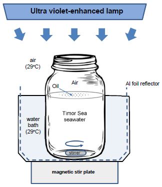
Figure 7: Schematic drawing of a microcosm used in the long-term weathering study. Oil (45 μL) was added to Timor Sea seawater (600 mL) maintained at 29°C, amended with indigenous bacteria and nutrients, continuously gently stirred, and irradiated (12 hr/day) for up to 84 days. ...
701 In describing the study, Dr Stout said:
[104] The long-term weathering study was more complicated as it needed to control multiple conditions – temperature, oxygen availability, water/oil movement, salinity, bacterial abundance, nutrient availability, ultra-violet light exposure, oil chemistry (i.e., the three forms of oil), and time – concurrently. However, this complexity was not unique to the Montara oil spill. Laboratory microcosm studies, such as my long-term weathering study, are the conventional way by which oil spill scientists study the rates and effects of weathering on spilled oil. Furthermore, microcosm studies yield weathered oils with compositions that resemble those of naturally-weathered oils, which indicates that the processes of biodegradation and photo-oxidation that occur in nature can be reproduced in the laboratory. Although the results obtained from my long-term weathering study are limited to the specific conditions of the study, those conditions were set to mimic, as practically as possible within the constraints of the laboratory, those that existed during the actual Montara oil spill. Therefore, it is my opinion that the rates and effects of weathering determined during the long-term weathering study reasonably represent those that existed in the days and weeks following the release of Montara oil into the Timor Sea
702 Dr Stout described the overall results of the study in respect of the three forms of oil as follows:
[112] ... The results of the study show:
(a) Weathering through continued evaporation (beyond that of the short-term study), biodegradation, and/or photo-oxidation commenced in all three forms of Montara oil within the first 7 days;
(b) Over the course of the 12-week study, two phases of long-term weathering were evident, being fastest and most extensive within the "early" phase (0-28 days), and slower and less extensive within the "late" phase (28-84 days);
(c) Throughout the study the chemically-dispersed Montara crude oil and its (non-dispersed) wax-depleted oil fraction weathered at comparable rates and to comparable extents, indicating dispersant (Slickgone NS) did not obviously increase (or inhibit) weathering, at least not at the sampling resolution of my study;
(d) The (non-dispersed) wax-enriched oil fraction weathered less and more slowly than the other two forms of oil studied, wherein weathering was likely slowed due to the wax's physical state; i.e., the smaller oil-water interface of the discrete, hydrophobic, floating waxy particles inhibited their weathering relative to the larger interfaces of the chemically- dispersed oil droplets or wax-depleted oil's thin sheen;
(e) Although evaporation initially contributed, biodegradation played the major role in loss of n-alkanes, while a combination of biodegradation and photo-oxidation led to the losses among the PAHs, mostly within the first 28 days;
(f) Biodegradation was ultimately so severe that the normally-recalcitrant biomarker compound, 17α(H),21β(H)-hopane, was partially depleted;
(g) Timor Sea water undoubtedly contains a consortium of indigenous, oil-degrading bacteria capable of biodegrading Montara oil.
703 Dr Stout summarised his conclusions as follows:
[115] In summary, my long-term weathering study showed that the combined effects of continued evaporation, biodegradation, and photo-oxidation dramatically changed the composition of Montara oil, and its wax-depleted and wax-enriched oil fractions derived from the oil, over the course of days and weeks. PAHs were rapidly and significantly reduced within the first 7 to 28 days, mostly (~80%) the first 7 days, albeit more slowly and to a lesser extent in the wax-rich residues (waxy particles) derived from the oil.
[116] Collectively, based upon the results of my short- and long-term oil weathering studies, the spilled Montara oil dramatically and rapidly changed its composition and concentrations due to weathering at/near the sea surface. These changes commenced quickly and proceeded rapidly, albeit somewhat more slowly in floating wax-rich residues than in chemically-dispersed oil droplets or floating sheens. The mass of the spilled oil was substantially reduced as aromatic hydrocarbons were eliminated from or markedly reduced (1) within hours in the case of MAHs and (2) mostly within the first 7 days and overwhelmingly within the first 28 days in the case of PAHs. …
[117] Because the conditions of my short- and long-term laboratory weathering studies mimicked, as practically as possible within the constraints of the laboratory, those conditions that existed during the actual Montara oil spill, it is my opinion that the changes in composition and concentrations of the Montara oil determined during these studies reasonably represent those that existed in the hours, days, and weeks following the release of Montara oil into the Timor Sea. This conclusion is further corroborated upon comparison of the laboratory results to those of field-collected oils and waxes...
704 Dr Stout theorised that the slower and overall lower depletions of PAHs in the floating waxy particles were due to the PAHs “inside” the particles being less available to bacteria and less exposed to UV radiation than dispersed oil droplets or floating sheens.
705 As I have already noted, the field-collected samples analysed by Leeder Consulting were of an unknown age when collected. This fact precluded any rigorous quantitative assessment of the rate(s) of weathering of the Montara oil during the spill.
706 Despite this shortcoming, Dr Stout considered the Leeder Consulting data to be important because, in his view, they provided corroboration of the wax-enrichment and weathering processes simulated in his laboratory studies. Dr Stout remarked that chromatograms of the “white waxy particles” collected at sea closely resembled those of his laboratory-produced, wax-enriched oil fractions after weathering in the laboratory for 70 to 84 days. He opined that the “white waxy particles” observed during the spill may have taken multiple weeks to be produced and that, owing to their semi-solid nature, were likely to be the most persistent form of Montara oil in the environment.
707 With regard to this persistence, Dr Stout said (in Annexure E to his principal report):
[125] My long-term weathering study showed that small waxy particles (~2 to 7 mm) physically lasted the duration of the study (84 days). Because weathering preferentially occurs on the exterior surface of the waxy particles, it follows that the rate of weathering of the waxy particles is inversely proportional to their size (surface area-to-volume ratio). Specifically, smaller waxy particles (larger surface area-to-volume ratio) would persist for a shorter period of time and vice versa. Physical processes (wave action or abrasion) would tend to reduce the particle size of waxes over time, eventually making smaller and smaller waxy particles, with larger and larger surface area- to-volume ratios, which would eventually weather completely.
708 Dr Stout also observed that Leeder Consulting had measured the concentrations of total aromatic hydrocarbons (>C7 to C35) in 13 field-collected samples and 16 PAHs in 42 field-collected samples. The data showed that, as the Montara oil weathered and/or became enriched in wax, the concentrations of total aromatic hydrocarbons and the measured PAHs decreased substantially. Dr Stout drew particular attention to the only “pure” wax sample measured by Leeder Consulting for aromatics, which retained only 1.6% of the total aromatic hydrocarbons (>C7 to C35) and 0% of the 16 PAHs. Dr Stout argued that this suggested that the loss of total aromatic hydrocarbons and PAHs from the “white waxy particles” observed during the spill likely exceeded the losses achieved in his laboratory weathering study.
709 Dr Stout also measured the concentrations of hydrocarbons, including monocyclic aromatic hydrocarbons or monoaromatic hydrocarbons (MAHs) and PAHs, dissolved in the seawater, or within oil droplets suspended in the seawater (particulate oil), potentially associated with three different forms of Montara oil (the WAF study). The three forms were: Montara-2 oil treated with dispersant (Slickgone NS); evaporated (21 wt%) Montara crude oil (obtained by evaporating fresh Montara-2 oil to the same degree as occurred after 7 days of evaporative weathering under Timor Sea temperature conditions); and an evaporated (7 wt%), wax-enriched oil fraction of Montara-2 oil. Dr Stout considered that these forms represented, respectively: fresh Montara oil sprayed with dispersant in conditions closest to the West Atlas platform; untreated, weathered Montara oil further from the platform; and the floating, solid, waxy residues observed in the field.
710 MAH concentrations were measured in the seawater directly, whereas PAH concentrations were measured in both the dissolved phase and particulate phase. Dr Stout referred to the dissolved and particulate phases as the water soluble fraction (WSF) and particulate oil fraction (POF), respectively. Taken together they comprise the water accommodated fraction (WAF).
711 It is important to understand that the WAF fraction is defined by the equation WAF = WSF + POF. By definition, the WAF fraction does not include the “floating oil”, including the floating wax-rich oil, that remained in the vessel containing the WAF fraction after harvesting to produce the WSF and POF fractions.
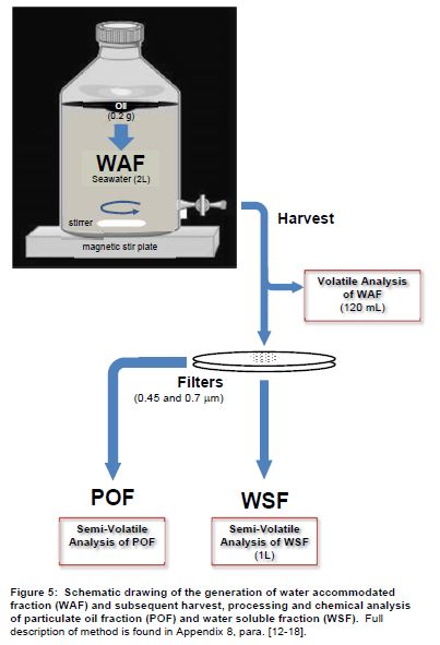
712 Dr Stout found that the seawater in contact with fresh Montara oil treated with dispersant contained the highest concentrations of all hydrocarbons in both dissolved and particulate phases. He said that this was due to a combination of this oil’s “freshness” and its dispersion into the water, which would have promoted dissolution of the oil’s more soluble compounds and the formation of suspended oil particles that remained in the water.
713 As this study was conducted at 29°C to mimic the average water temperature in the Timor Sea throughout the spill, the wax-enriched oil fraction remained as a solid, floating wax-rich particle throughout the experiment. Nonetheless, seawater in contact with this particle contained 814µg/L of MAHs, comprising mostly of BTEX (619µg/L), which apparently dissolved into the seawater in contact with the particle. PAHs were also dissolved into the seawater in contact with the particle (348µg/L), albeit in lower concentrations than the other two forms of oil studied. The PAHs in the wax-enriched oil fraction mostly comprised dissolved naphthalenes in the WSF (283µg/L).
714 It is to be noted that MAHs and PAHs are typically associated with toxic effects on marine biota. The objective of this study was to produce data of use to others to assess the potential toxicological impact(s) of the Montara oil spill on aquatic organisms.
Criticisms of Dr Stout’s long-term weathering study
715 Professor Ball expressed concern about the way in which Dr Stout had produced his wax-enriched fraction on which he conducted his long-term weathering study. He observed that spinning the oil at high velocity to produce the wax-enriched oil fraction was not, to his knowledge, a published and validated technique, and was not a process to which the Montara oil was subjected during the spill. He observed that Dr Stout’s opinion that the wax-enriched oil fraction was “reasonably representative” of the solid, wax-rich residues that were observed floating at sea during the spill, was an undefined standard involving a subjective judgment based on his (Dr Stout’s) visualisation of photographic images and the fact that the product he formed was a solid at room temperature. Professor Ball expressed surprise that, given that Dr Stout had 18 months to conduct his analyses, an 18-month weathering experiment had not been performed.
716 In the Joint Report on Chemical Composition, the experts agreed that Dr Stout’s long-term weathering study did not replicate (in the sense of mimic) the dissolution of Montara oil through weathering. This was because the study was conducted using 600 ml of seawater in glass containers, such as depicted above. They said that the glass containers prohibited the diffusion/dispersion of any dissolved chemicals away from the oil in the container. They observed that, in an open ocean, with an “infinite” volume of water, these dissolved chemicals would have been allowed to move away from the oil. As Professor Ball put it in a responding report dated 4 May 2019, Dr Stout:
5.4 … designed a simple experiment, with only a temperature and agitation being considered as environmental factors. Other key factors such as the impact of tides, winds and the presence of macro-flora and -fauna were outside the scope of this study.
717 Also, Professor Ball and Dr Fingas did not consider that Dr Stout’s long-term weathering study replicated the biodegradation and photo-oxidation of Montara oil through weathering. Dr Fingas commented that Dr Stout’s study provided no comparison point with the weathering of fresh Montara oil. Thus, what is not known from the study are the properties of the oil at different weathering stages; anything about unaltered Montara oil as it weathers past 7 days; the oil’s true viscosity at standard temperatures; and whether separation of the oil occurred and, if so, what happened to the separated fractions. Dr Fingas also commented on the fact that, despite Dr Stout’s long-term weathering study, little is known about how the appearance of the oil (for example, whether it is white, green, orange, yellow, or brown) is related to its chemical and physical properties.
718 Like Dr Fingas, Professor Ball commented on the absence of a control using fresh Montara oil to compare results over the 84 days of the experiment, although he noted that other controls were used in the study. Professor Ball described this as a significant flaw in the study. Further, a parallel experiment would have allowed the measurement over time of important parameters such as wax content, pour point, viscosity, dispersability, and toxicity.
719 Professor Ball also commented that Dr Stout’s biodegradation work involved isolation of a specific hydrocarbon-degrading microorganism from a pre-enriched seawater sample, which was then added to the seawater at the beginning of the long-term study. Professor Ball said that this addition would significantly impact on the biodegradation process. Further, after 21 days of incubation a further addition of the microorganism was made. Professor Ball argued that this was a bioaugmentation event aimed at enhancing the biodegradation of the petrogenic hydrocarbons. He pointed out that, as there was no estimation of the actual numbers or activity of the specific isolate in the fresh seawater, it was not possible to assess the impact of these additions on the biodegradation processes. Indeed, in his responding report of 4 May 2019, Professor Ball argued that Dr Stout’s comments on biodegradation were based purely on chemical fingerprinting data.
720 In relation to Dr Stout’s comments concerning “pure” wax samples, Professor Ball noted that Dr Stout had provided no definition of “pure”. He noted further that Dr Stout’s experiments showed that even after “12 weeks incubation”, the concentration of PAHs remaining in the wax was 5,320 µg/g, representing 86% degradation (I note that in Table 9 to his report dated 12 March 2019, Dr Stout recorded total remaining PAHs as 6,204 µg/g). Professor Ball said that this wax should not be deemed to be “pure”.
721 Dr Fingas made a similar observation. He said that Dr Stout had repeatedly stated that extensive weathering would result in “pure” wax. Dr Fingas noted that one sample showed a large wax content (I assume this is the sample in the Leeder Consulting reports that Dr Stout relied on), but several other samples did not. He commented that the predominance of the evidence shows that wax concentration simply follows a weathering pattern. Dr Fingas observed that Dr Stout’s results showed that, after 84 days of biodegradation and evaporation, the remaining oil from the wax-enriched oil fraction consisted of 28% saturated hydrocarbons including wax, 1.4% of aromatics, and 71% of other compounds. Thus, the portion containing the waxes only constituted 28% of the mass. Many of the larger aromatics, known for their persistence and toxicity, were retained in that fraction.
722 Dr Stout defended his long-term weathering study. He contended that laboratory weathering studies are commonly used in oil spill science to understand the weathering that occurs. He said that the conditions of his long-term study mimicked, as practically as possible within the constraints of the laboratory, those conditions that existed during the actual Montara oil spill, by using indigenous bacteria in a concentration that occurred naturally in the Timor Sea, and artificial sunlight. That said, Dr Stout remarked that biodegradation and photo-oxidation did not “wait” to commence only after the spilled oil had evaporated for 7 days, as did his study. Rather, in the real world, bacteria and sunlight would begin acting on the spilled oil simultaneously as it evaporated. In making this observation, Dr Stout was expressing caution that his measurements were likely to have underestimated the extent of weathering on the composition of the spilled oil and the concentrations of hydrocarbons in that oil.
723 Dr Stout also acknowledged that he could not replicate the process of wax-agglomeration and separation during his long-term study. He repeated his earlier contention that one of the Leeder Reports reported on floating wax-rich particles that exhibited a greater loss of PAHs than he was able to achieve in the laboratory.
724 Dr Stout also acknowledged that the rates of weathering of different forms of Montara oil during the spill would have varied and that the rates he observed were specific to the particular fractions he studied. He argued, however, that the specific wax-enriched oil fraction he studied was but one fraction along a “continuum of increasing wax-enriched particles that formed during the actual spill”.
725 Dr Stout accepted that chemically-dispersed droplets would not have been able to diffuse/dilute within the glass vessels he had used, but argued that this meant it was likely that chemically-dispersed Montara oil weathered more quickly during the actual spill than he observed in his long-term study. On the other hand, he said it was likely that thicker floating oil slicks, not thin sheens, weathered more slowly during the oil spill than the sheens he used in his study.
726 With respect to the non-inclusion of fresh Montara oil in his long-term study, Dr Stout argued that, as evaporation quickly altered the chemical composition of spilled Montara oil, it was “completely reasonable” that he should commence his long-term study with evaporated oil, not fresh oil.
727 With respect to the addition of the bacteria to his study, Dr Stout stressed that only indigenous bacteria isolated from the Timor Sea had been added using standard microbiological procedures. He explained that there was nothing special about the bacteria he had used and that such additions were not uncommon in laboratory weathering studies because of the “difficulty-to-impossibility” of keeping bacteria alive during the shipping of seawater samples, in this case from Australia to the United States of America. Thus, he argued, the biodegradation during his long-term study was not significantly affected by the addition of live bacteria at their real-world concentration.
Conclusions on Dr Stout’s long-term weathering study
728 Dr Stout’s long-term weathering study was an attempt to mimic, in the laboratory, the chemical composition of spilled Montara oil that had weathered over an 84 day period. His study was based on the three forms of Montara-2 oil he had prepared. The applicant did not challenge the skill with which this work was carried out or the actual results that were obtained. What the applicant did challenge, through Professor Ball and Dr Fingas, was whether the results obtained could be accepted as reliably representing the actual chemical composition of weathered Montara oil given that the experiments were: (a) benchtop experiments; and (b) carried out, in the case of the wax-enriched oil fraction, on starting materials that had been derived from a process (chilled centrifugation) that was certainly not a process to which the spilled Montara oil had been subjected in the field. The latter point was the gravamen of Professor Ball’s and Dr Fingas’ criticism, that no control using fresh Montara oil had been provided to show that the wax-enriched fraction was, in fact, representative of the spilled oil, or any part of the spilled oil, that had weathered.
729 Dr Stout argued that his wax-enriched oil fraction was one fraction along a continuum of increasing wax-enriched particles that formed during the actual spill. He also argued, based on one of the Leeder Reports, that the loss of PAHs observed from his study was likely to be conservative.
730 Even though laboratory studies have their limitations in mimicking the real world, as Dr Stout himself acknowledged, I certainly would not dismiss his work because it was based on such studies. However, there is no reason to think that, at the time of the spill, the Montara oil separated into the particular wax-depleted and the wax-enriched fractions which Dr Stout used as two of the starting points for his long-term weathering study. It is, of course, possible that the wax-enriched fraction obtained through chilled centrifugation was representative of some part of the spilled oil that had weathered. I could not say otherwise. Indeed, the Leeder chromatograms provide some broad support for that conclusion. But if Dr Stout’s wax-enriched fraction was, as he argued, on the continuum of increasing wax-enriched particles that formed during the actual spill then, absent a control, there is no objective standard by which it can be known where that fraction sat on that continuum or to what extent it might represent the chemical composition of the spilled oil that, on the applicant’s case, reached the shores of Rote/Kupang. This is the principal reservation that I have with the results of the long-term weathering study carried out with respect to the wax-enriched fraction.
731 I accept that, as a general trend, the weathering of the oil spilled from the H1 Well would have resulted in the rapid loss or depletion of MAHs and PAHs. But the three forms of oil studied by Dr Stout do not represent all the weathered states in which the spilled oil might have reached the coastal waters of the Rote/Kupang region. Therefore, his results are not conclusive of the PAHs present in that oil. I note, in any event, that in Dr Stout’s long-term study some PAHs remained in the three forms of oil after 28 days, with the weathering of the remaining PAHs proceeding only incrementally, particularly in the wax-enriched fraction.
732 Another reservation I have with respect to the long-term study is the addition of bacteria, including after 21 days, to the materials that Dr Stout was studying. The reason why the bacteria were added has been explained. I do not for one moment think that they were added to deliberately enhance bioaugmentation. Based on Dr Stout’s undoubted experience, I accept his evidence that the addition of such bacteria is not uncommon in laboratory weathering studies. However, no estimation of the actual numbers of activity of the specific isolate in fresh seawater was carried out. It is not possible to assess the impact of this addition on the biodegradation process. Therefore, the extent to which that addition might have influenced the results that were obtained does introduce a further element of uncertainty as to the extent to which the long-term study did, in fact, mimic the weathering of Montara oil that took place during the course of the spill.
733 The applicant submitted that the likely consequence of Dr Stout adding bacteria is that a greater amount of oil was biodegraded than would have been the case with the oil that was spilled from the H1 Well, thereby reducing the quantities of compounds present in the studied fractions over the entire course of the 84 day long-term weathering experiment. The applicant submitted that to the extent that the Toxic Units Model deployed by Dr Maki, discussed below, included data from the long-term weathering study to determine the acute and chronic toxicity of the Montara oil on particular days, it underestimates the toxicity of the oil.
734 Having regard to the other evidence before me, the reservations I have expressed do not, ultimately, affect the conclusions to which I have come on the principal factual questions for decision in this case—whether Montara oil spilled from the H1 Well blowout reached the Rote/Kupang region and, if so, whether that oil damaged the seaweed crops in that region. This is so even though Dr Stout’s work was directed, in part, to assist in determining the toxicity of fresh and weathered Montara oil, a topic to which I will return.
735 One matter that is not in doubt is that the wax content of Montara oil increases with weathering. As it weathers, Montara oil will result in the formation, and separation from the oil, of wax-rich residues which, in physical appearance, can be described by expressions such as blocks, clumps, balls, and globules. These aggregates will be variously coloured, depending on the extent of the weathering that takes place.
736 At this point, it is convenient to discuss analyses carried out by LEMIGAS. As I have already noted, LEMIGAS is an Indonesian governmental oil and gas research organisation. The analyses were carried out on material (sediments, coral, tar balls, and mangrove root) collected from certain locations in the Rote/Kupang region in December 2017 and April 2019, long after the Montara oil spill. Those undertaking the analyses concluded that four of the samples collected in 2017 and 2019 contained Montara oil.
737 The LEMIGAS analyses were introduced into evidence by an unusual route. The applicant served the LEMIGAS analyses on the respondent. Dr Fingas also prepared a report in which he concluded that even more samples taken by LEMIGAS showed, or possibly showed, the presence of Montara oil. Specifically, Dr Fingas concluded that, when properly analysed, the LEMIGAS data revealed four samples showing the presence of Montara oil and eight samples showing the possible presence of Montara oil. In a responding report, Dr Stout criticised the LEMIGAS analyses and findings, as well as Dr Fingas’ findings. In the end, the applicant made a forensic decision not to rely on the LEMIGAS analyses. This decision was made on the basis that, when all of the evidence on this particular topic was taken into account, the Court was unlikely to conclude, on the balance of probabilities, that the samples taken by LEMIGAS in December 2017 and April 2019 contained Montara oil. I note for completeness that LEMIGAS also analysed three tar balls sampled in 2009 (which had been collected approximately 150 kms north of the Montara wellhead platform) and concluded that they contained Montara oil. There is no dispute about that finding.
738 The respondent took a different view of the forensic utility of this evidence and decided to pursue the topic. It tendered, without objection, certain annexures from a report prepared by LEMIGAS, and an expert report from Dr Stout dated 25 September 2019. The applicant tendered an amended report from Dr Fingas dated 3 December 2019.
739 Dr Stout analysed the LEMIGAS data using a protocol prepared by the Centre for European Norms called CEN 15522 – 2. Dr Stout’s evidence was that this protocol provides the state-of-the-art methodology for oil “fingerprinting”. “Fingerprinting” oil involves comparing the ratios of certain, highly-specific biomarkers present in the oil with the known ratios of those biomarkers in a reference oil (here, Montara oil). One of the ratios used by LEMIGAS, and which featured in the evidence before me, was C24 tetracyclic terpane/ C30-diahopane. In its analyses, LEMIGAS referred to C24 tetracyclic terpane as compound “8” and to C30-diahopane as compound “D”.
740 Using the CEN 15522 – 2 protocol, Dr Stout concluded that none of the samples collected by LEMIGAS in December 2017 and April 2019 contained Montara oil. LEMIGAS did not use this protocol or, it seems, any similarly known protocol.
741 With respect to the LEMIGAS analyses, Dr Stout said that, because of insufficient quality control, the collected chemical fingerprinting data lacked reliability at the outset. The data did not meet typical environmental geochemistry standards. Further, according to Dr Stout, the protocol that was used to compare the samples’ fingerprints with Montara oil’s fingerprint was poorly explained and over-simplistic. He said that it did not meet the scientific rigour of any of the published oil spill identification protocols. Further, according to Dr Stout, those undertaking the LEMIGAS analyses ignored key diagnostic features of Montara oil when concluding that the four samples “matched” Montara oil.
742 Dr Stout also observed that the concentrations of TPHs measured by LEMIGAS were likely to be biased (high) due to the presence of elemental sulphur and/or the presence of naturally-occurring biogenic hydrocarbons. Those undertaking the analyses appeared to have assumed that TPHs represent only petroleum hydrocarbons. As Dr Stout explained:
[81] The problem of biogenic hydrocarbons is very important when measuring TPH in soils or sediments. This is because some soils or sediments, such as a seagrass bed or mangrove forest, will contain an abundance of decaying plant, algae, and bacteria biomass. This decaying biomass is what makes such soils/sediments dark in color. This decaying biomass contains naturally-occurring hydrocarbon derived from plant waxes, terpenes, fats, and lipids that were part of the plants, algae, and bacteria when they were alive. These hydrocarbons are soluble in n-hexane and therefore contribute to TPH, even though they are not petroleum. This is a well-recognized issue in environmental geochemistry since sometimes “clean” sediments are erroneously considered to be contaminated with petroleum, when they are not.
743 Dr Stout said that simply detecting TPHs in an ad hoc collection of sediments is not a reliable indicator of oil contamination. In any event, Dr Stout said that, given the low concentrations of TPHs measured in most of the collected sediments, the actual concentrations of any oil in each sample was equivocal (i.e., clearly low and perhaps absent).
744 In summary, Dr Stout concluded that:
[12] … the limited ad hoc studies conducted in 2017 and 2019 provide no chemical evidence of any impact to the shorelines of West Timor, Semau Island, and Rote Island by Montara crude oil. The results do show multiple “non-Montara” oils are present at mostly low concentrations throughout the area – likely owing to pervasive natural oil seeps in the region.
745 Dr Stout’s criticism of Dr Fingas’ evaluation of the LEMIGAS data was more trenchant. Dr Fingas employed regression analysis to compare the LEMIGAS biomarker ratios. Dr Stout described this method as “unique, unpublished, single-tiered and arbitrary”. Dr Stout observed that no past or current oil spill protocols rely on Dr Fingas’ method and that Dr Fingas himself had cited no supporting references in the oil spill literature. Dr Stout argued that the “matches” that Dr Fingas achieved when carrying out his evaluation were meaningless. He argued that, by Dr Fingas’ method, false positives were easily obtained. He argued that Dr Fingas had used duplicated, re-scaled and non-diagnostic ratios and that Dr Fingas had also ignored, or diluted the importance of, some “key diagnostic features”.
746 In response, Dr Fingas maintained his findings. He disputed that he had used duplicated ratios. He also emphasised that one problem with oil “fingerprinting” was that the ratios of the biomarkers used for comparison change with weathering. Dr Fingas said that there are no current statistical methods to correct for the effects of the long-term weathering on these biomarkers. He argued that the biomarkers that Dr Stout had used are good for short-term comparison (meaning “good” for days or maybe weeks). He said that highly-weathered samples of the same oil are hard to identify using these biomarkers. He said that, in the case of the LEMIGAS samples, there may have been extensive biodegradation of the biomarkers that were used for comparison and that, in fact, more of the LEMIGAS samples may have contained Montara oil.
747 For his part, Dr Stout said:
65 I considered the possible effect of weathering of the Montara oil on its biomarker distribution even though most biomarkers are considered extremely resistant to weathering on environmental timescales. Some of the “key” triterpene biomarkers I consider to be particularly diagnostic of the Montara oil are actually known for their resistance to weathering. For example, the C24 tetracyclic terpane … and C30-diahopane … are both reportedly even more resistant to biodegradation than hopanes. Thus, the absence or reduced relative abundances of one or both these two “key” biomarkers relative to the Montara oil cannot be reasonably explained by biodegradation. Therefore, differences in these biomarkers’ relative abundances (versus the Montara oil) indicates the presence of a different type(s) of oil in many samples …
748 Based on Dr Stout’s evidence, I have strong reservations that the LEMIGAS analyses are reliable for the various reasons he advanced. I am certainly not satisfied that it has been shown that the samples collected by LEMIGAS in 2017 and 2019 did contain Montara oil.
749 Further, on this topic I prefer the rigour of Dr Stout’s methodology and analysis over Dr Fingas’ analysis. I am not persuaded that Dr Fingas’ regression analysis possessed the rigour to enable firm conclusions to be drawn. Further, Dr Fingas’ analysis did not account for the deficiencies in sampling to which Dr Stout referred. In other words, Dr Fingas’ analysis could be no better than the sampling that LEMIGAS carried out. In reaching my acceptance of Dr Stout’s analysis, I do not ignore the possibility that the weathering of biomarkers may have influenced the negative findings he made. However, I also think that it would be entirely speculative for me to conclude that, but for the effects of weathering, the samples would have shown the presence of Montara oil.
750 Plainly, it does not follow from these findings that Montara oil did not reach the shores of Rote/Kupang in the latter part of 2009 as a result of the H1 Well blowout. My conclusion is that the LEMIGAS analyses and Dr Fingas’ analysis do not establish the converse proposition.
751 Sedeoen is a small village on the western coastline of Rote. It stretches from the coast back (for about 1 km) to the main road that goes to Ba’a, the main town of Rote. The beach at Sedeoen is approximately 2 to 3 km north of Nemberala. It is a west-facing, sandy beach that leads to a tidal flat that extends for about 300 m before it reaches deeper water. There is a reef (called the Bombora) that is about 500 to 600 m from the high tide mark. There is another reef about 300 m further out, where some waves break. To the north and south there is a flat reef that runs all the way along the western end of Rote.
752 In 2009, Adrian Sibert lived at Sedeoen. He had a boat which he moored at the beach. In late September 2009, he was visiting Nemberala. He heard about oil washing up on the beach. He went to investigate. He gave this evidence:
45. ... I walked to Nemberela beach in front of Anugerah homestay. This was about a five minute walk from Johnny's bar. By the time I got to the beach it was late afternoon, around 5 to 5.30 pm, just before sunset. I saw these oily mustard coloured globules on the beach along the tide line mark for as far as you could see. I could also see the same globules in the water within the lagoon in front of the Anugerah homestay. I walked along the beach for 100 metres observing these globules. I felt the globules washed up on the beach. They were leaving shiny patterns like a rainbow in the light of the setting sun. I had never seen anything like the globules before.
753 The next morning he decided to go fishing at Sedeoen. When he arrived at the beach, where his boat was moored, he saw globules along the high tide mark, the same as he had seen the previous evening at Nemberala. When he ventured out in his boat, about 50 m from the shore, he noticed foamy patches floating on the surface of the water. He said:
51. I looked at the patches of foam more closely. I could see two different substances and dead fish within the white foam. The foam was floating on top, up above the surface water level. The pale milky-mustardy coloured globules were floating underneath the white foam and within the surface area covered by the foam. The white foam was a brighter colour than the globules. The globules were still floating but they were at the surface level of the water with the fish. There were about six dead fish floating in the patch of foam, which covered an area of about six metres in diameter.
754 Mr Sibert decided to take a sample. He went back to the beach where he picked up an empty 500 ml plastic water bottle. He said it was not unusual to find bottles on the beach at Sedeoen because the seaweed farmers used them as floats. He then returned to his boat and motored offshore. He said:
62. In between the two reefs out the front of my property I could see a concentration of the foam patches. I could see many dead mackerel around half a kilo in weight and 20 cm in length and some dead bonito and oily globules floating in a large foam patch in that area. I decided to take a sample of the water from that particular patch of foam.
…
65. In the middle of this foam patch I used my gaff to try to spread the foam apart to expose the globules underneath. My gaff is just a stick with a big hook on it attached to the end that I made for my fishing. I used my gaff to push the foam away to get a water sample with the globules in it.
…
67. I placed the water bottle into the water to get the sample and I pushed three to four of the globules into the bottle for collection. When the globules were in the bottle they floated to the top and joined together.
755 At the suggestion of his friend Edwin Larrick, Mr Sibert wanted to have the contents of the bottle analysed in Australia. He thought it important that he try to seal the bottle as best he could. He wrapped it in plastic film. On the recommendation of a friend in Kupang, he (or Mr Larrick) gave the sealed bottle to Miriam Chalvet. The sealed bottle then found its way into the hands of a Richard Flax, sometime in November 2009. It appears that Mr Flax was living in Bali at the time. Mr Flax decanted the contents of the bottle into a metal flask. The flask was then transported to Australia by his wife, who took it to their residence in Cottesloe, Western Australia, where it was then either collected by a representative of the Greens Party in Perth or delivered to Senator Siewart’s office by Mr Flax’s wife.
756 On 19 January 2010, the flask was received by Leeder Consulting for testing. On receipt, Leeder Consulting observed that the flask contained mostly seawater with some botanical matter. On analysis, it was found to contain a very small amount of highly weathered hydrocarbons. However, the whole of oil ratios of the sample did not match the whole of oil ratios of fresh Montara crude oil. The sample was therefore eliminated from further analysis.
757 Leeder Consulting received two other samples on 19 January 2010 which, on testing, were found to contain Montara oil. One of these samples was delivered in a plastic 500 ml bottle that was wrapped in plastic film. It was observed to contain mostly water with some wax particles adhering to the plastic. Mr Sibert believed that this bottle was the sample he had collected. He maintained this belief under cross-examination. There is no suggestion that Mr Sibert gave his evidence untruthfully. However, the applicant did not advance a case that the contents of the sealed plastic bottle received by Leeder Consulting on 19 January 2010 was the sealed bottle containing the sample taken by Mr Sibert in late September 2009.
758 The respondent relies on the testing of the contents of the flask received by Leeder Consulting on 19 January 2010 as showing that the sample, as collected by Mr Sibert in late September 2009, did not contain Montara oil. I am not prepared to make that finding.
759 First, Mr Sibert’s description of the sample he took in late September 2009, which contained globules and foam, does not match Leeder Consulting’s observation of the sample it received in January 2010. Something had caused a change. Secondly, Leeder Consulting noted that each of the containers for the three samples it received in January 2010 was inappropriate for the sampling of oil spills. Thirdly, I have no confidence that the sample taken by Mr Sibert was otherwise stored under appropriate conditions which would enable the sample, as collected, to be scientifically analysed. Fourthly, the sample taken by Mr Sibert was not analysed for more than (approximately) 3 months after collection. I have no way of telling what the effects of biodegradation may have been over that time.
760 In short, the integrity of the sample taken by Mr Sibert and analysed by Leeder Consulting is seriously in question—so much so that no sound factual findings can be made about whether it contained or did not contain Montara oil at the point of collection in late September 2009.
761 I am fortified in this view having regard to the following evidence given by Dr Coelho in relation to other samples that were collected and analysed at the time of the Montara oil spill:
Water Sampling During Montara
…
There are very specific sampling protocols required for handling oil samples, such as proper submerging of the sampling device and transfer of samples to the storage container; using amber bottles to prevent UV degradation of the sample during transport; preserving volatiles by ensuring that there is no headspace (trapped air) in the bottle; preserving and possibly spiking the sample (varies based on analytical protocols by individual labs); ensuring proper chain of custody; and refrigerating samples immediately. These protocols exist because hydrocarbon samples can continue to degrade if not properly stored. ...
762 Dr Coelho said that poor sampling and the incorrect storage of samples negates any hydrocarbon analysis data derived from them.
Expert commentary on the lay observations of oil
763 Professor Ball was provided with a Schedule of Observations prepared as at 17 September 2018. It appears to be a compilation of affidavits obtained on behalf of the applicant as well as certain contemporaneous emails reporting on observations of oil.
764 Professor Ball was asked to assume that the observations were of Montara crude oil, unless he was of the view that they could not be, or were unlikely to be, of Montara crude oil. He was then asked to identify the likely properties of the observed oil; its behaviour and likely effects on the environment; and its persistence in the environment.
765 In his report dated 23 October 2018, Professor Ball identified, from this material, a number of features and effects which he characterised by reference to the following headings: Weathering; Adhesion; Smell; Impact on seaweed; Impact on sea life; Impact on humans; Transfer through food chain; Persistence of Montara crude oil; and Sea foam.
766 Professor Ball said:
10.2 Overall there is a remarkable similarity in the observations described regarding the properties of the weathered Montara crude oil. Often the same descriptions are presented but described in different ways. However there is sufficient clarity to identify the key features of the statement. This does not mean that the observations all describe the same features. Rather the array of descriptions reflect the range of weathering states that have been described through the sampling and analysis of Montara crude oil samples throughout the oil spill period. All the descriptions are consistent with the expected behaviour of Montara crude oil during the weathering process. It is not surprising that the Montara crude oil arriving around Indonesia was in different weathering states according to its age and exposure to environmental and chemical conditions. I am in no doubt that the oil described by witnesses was weathered Montara crude oil.
767 Two matters should be noted. The first matter to note is that not all the affidavits comprising the Schedule of Observations were read as evidence at the hearing. With respect to those affidavits that were read, not all the paragraphs were read. Further, a number of deponents gave oral evidence of their observations at the hearing.
768 The second matter to note is that, Professor Ball was asked to assume that the observations with which he was provided were of Montara oil unless he could, in effect, reject that possibility. Professor Ball did not reject that possibility. In the end result, he treated all the observations as characterising Montara oil.
769 In light of these matters, Professor Ball’s opinions on this topic must be treated with caution if they are used as a step to establishing that the substances that the lay observers saw were Montara oil in some form. That said, there was no objection to the tender of his report dated 23 October 2018, or to any of his other reports dealing with this topic. Through the process of concurrent evidence (involving, on this topic, Professor Ball and Dr Fingas, Dr Taylor and Dr Maki), and subsequent cross-examination, evidence emerged which assists in making findings as to whether the observations of the lay witnesses (which I have summarised in Schedule C to these reasons) were of Montara oil.
770 Dr Fingas contributed to the evidence on this topic. He said that the appearance of oils can be affected by their wax content. He said that the aerial observations of Montara oil near the Indonesian border included brown, white, metallic, and orange colours. Dr Fingas reviewed 34 AMSA aerial observation documents, comprising videos, photographs or screenshots and surveillance flight reports relating to, amongst other things, AMSA flights taken on 13, 16, and 18 September and 1 October 2009. He said that the videos, in particular, are helpful in that they show that the largest number of slicks are described as brown, metallic, orange or white. The videos are typically near or over the Indonesian border.
771 Dr Fingas prepared a table of aerial and surface observations (including the observations of the seaweed farmers) identifying the colours that were observed at various distances from the H1 Well and at Rote. He noted that the observed colours from near the H1 Well (at distances <10 km and 10 to 100 km) carried through to the observed colours at Rote.
772 Dr Fingas noted that one of the “colours” observed was “rainbow colours”. Dr Fingas said that rainbow colours derive from the spreading of “metallic” slicks and that “metallic” slicks were frequently observed in Indonesian waters by AMSA aerial observers. Once near shore, slicks are likely to spread out to thinner slicks; for example, “metallic” slicks will spread out to “rainbow” slicks. Dr Fingas said that a “metallic” slick contains 10 times as much oil as a “rainbow” slick. Thus, a “rainbow” slick observed near Rote may be 10 times larger in area than the “metallic” slick. He opined that a “rainbow” slick near Rote is highly likely if “metallic” slicks are observed in close proximity to the Rote coastline.
773 Dr Fingas also gave evidence about “wax balls” (also called “tar balls”). These are collections of oil residues. Waxy oils are prone to form these balls. They are not visible from the air. They are not visible far from a boat. Dr Fingas said that, most often, one only sees tar balls when they land on a beach. They can contain oil and, if breached, can release that oil. Some of the seaweed farmers say they saw these balls.
774 Dr Fingas said that oil can be transported a long distance and still have an odour. He said that tar balls that are opened up can yield odours, which not only come from some oil components but also degrading oil components.
775 Dr Taylor, who was called for the respondents, was provided with a Summary of Observations of Oil as well as a collection of other materials, including the Schedule of Observations provided to Professor Ball.
776 The Summary of Observations of Oil appears to have been prepared by the respondent’s solicitors for the purpose of assisting Dr Taylor in preparing his expert report dated 4 September 2019. It contains extracts from the affidavits of lay witnesses that were read at the hearing together with extracts from the transcript where the witness also gave oral evidence. The collection of other materials included the reports of other experts (in particular, Dr Stout); AMSA Operational Monitoring Studies; several reports by Leeder Consulting; and APASA and other monitoring studies of the spill.
777 Dr Taylor was asked to address this question:
Whether and, if so, to what extent, the observations of phenomena near the coastline of Nusa Tenggara Timor and in the surrounding Timor Sea in about September 2009 set out in the summary of lay witness observations of oil in this proceeding are consistent with fresh or weathered Montara oil and /or are consistent with any other phenomena.
778 This is a different question to the question that Professor Ball was asked.
779 In addressing this question, Dr Taylor reviewed the observations of oiling and slicks that were undertaken by the trained observers (his Table 1 – Images and descriptions of Montara crude oil from overflights and samples). He then compared those observations with the observations in the summary of Observations of Oil and prepared a table identifying the lay witnesses’ observations that were consistent with Montara oil and the observations that appeared to him to be inconsistent with Montara oil (his Table 2 – Comments on summary table of oiling observations).
780 Dr Taylor explained the reason for this approach:
19. To address the above question, I have reviewed and summarized oiling observations of the slicks related to the Montara oil captured by aerial observers and personnel collecting samples of oil and underlying water from vessels operating in the spill area. It is my expert opinion that the observations made by personnel conducting overflights and collecting samples of oil in the field are more reliable than those of untrained people. An important aspect of understanding what appearance and forms oil may take as it weathers following a spill is to familiarize observers with what the oil looks like near the source and progressively farther away from the source (that is, more weathered).
20. In my experience based on responding to multiple oil spills, untrained people often report what they believe to be oil, particularly when they know a spill has happened. Part of the work that I, or personnel working for me, have had to do is to deploy and verify if, in fact, reports received of oiling are actually from the spill we are working on and not natural phenomena such as biological sheens, foams, diatoms blooms, or a different oil unrelated to the particular spill.
21. The field observations from overflights and sample collection overall are consistent with the appearance of fresh to weathered Montara oil documented generally as brown (fresh) to a brown wax-depleted liquid and a gold (yellowish brown) wax-enriched fraction from the laboratory weathering tests provided in Dr. Stout’s report. As Dr. Stout further notes: “Eventually, the spilled Montara oil formed a nearly “pure” wax and were described by Leeder Consulting as “white-waxy particles” during their collection at sea.”
22. …
23. Aerial observations recorded of oil appearance from overflights and from sample collection activities that I have reviewed are summarized in Table 1. Examples of oil appearance at distinct distances from the well head site are provided in Figure 1 ... It is my opinion that these descriptions and photographs of the fresh to weathered Montara oil are the most reliable indicators of the oil appearance near source and at far-field locations.
781 In his oral presentation to the Court, Dr Taylor said:
I relied tremendously on trained observers and the people that are out there on a regular basis because they see that oil on a recurring basis and they also have the benefit of seeing the oil near the wellhead source as well as farther away from the source. And trained observers usually have – are able to discern phenomena that may look like oil but is not oil. And so sometimes they can separate those two things. So the field – the field observers are one of the primary mechanisms I relied on for what that weathered Montara oil would look like.
782 It is convenient to interpose, at this point, some of the lay observations that Professor Ball considered to be consistent with the features of Montara oil, which Dr Taylor and Dr Maki considered to be contentious.
783 Professor Ball noted that a number of witnesses had commented on the smell of the substances they identified as oil. Professor Ball remarked that the descriptions of smell varied from kerosene smells, to engine and lubricating oil smells. He said that this was indicative of variable weathering, with the reports of engine and lubricating oil smells indicative of heavy weathering.
784 As to this, Dr Taylor noted Dr Stout’s characterisation (based on his long-term weathering studies) of far-field weathered Montara oil residues as primarily “pure” wax. Based on Dr Stout’s characterisation, Dr Taylor said:
25. Given the lack of BTEX compounds and the depletion of aromatics and prevalence of waxes in weathered Montara oil, and based on my experience with fresh to very weathered oils (one or more months of exposure) on multiple spills, I expect little to no odour for far-field weathered waxy Montara particle residues and certainly no strong fuel or petroleum odours.
785 Dr Taylor also noted that a far-field sample collected at Browse Island by trained observers, which was later analysed by Leeder Consulting as containing traces of Montara oil, was said not to have any odour.
786 Another contentious feature referred to by Professor Ball concerns the presence of foam. Professor Ball said:
10.1 …
(i) … A number of depositions described a sea foam being present. Sea foam, ocean foam, beach foam, or spume is a type of foam created by the agitation of seawater, particularly when it contains higher concentrations of dissolved organic matter (including proteins, lignins, and lipids) derived from sources such as the offshore breakdown of algal blooms. These compounds can act as surfactants or foaming agents. As the seawater is churned by breaking waves in the surf zone adjacent to the shore, the presence of these surfactants under these turbulent conditions traps air, forming persistent bubbles that stick to each other through surface tension. Due to its low density and persistence, foam can be blown by strong on-shore winds from the beach face inland. The origin of the surfactants is unknown but there are two possibilities:
• The biological material that has been damaged thereby releasing the biological surfactants; and
• The presence of surfactants from dispersants remaining within the oil.
787 Dr Taylor remarked on the fact that samples of foam collected at Ashmore and Browse Islands had been characterised as primarily biogenic material with “trace to no oil”.
788 With reference to the description of Montara oil by trained observers, Dr Taylor said that his expectations of the descriptions of oil, consistent with Montara oil, would be oil:
28. … ranging from thick to thin, dark orange, orange to some brown, coherent to dispersed slicks; yellow or gold emulsified slicks; khaki slicks; to white or grey waxy patches, patties, or particles. None of the observations listed in Table 1 described the oil as occurring as a froth or foam. Sheens are noted as predominately as silver sheen although rainbow sheen was noted for a few samples collected within 6 to 11 km of the well site. The dispersed, white waxy particulates are what I would expect to find for far-field weathered Montara oil, with little to no odour, possibly associated with very limited rainbow sheen (along the edges of concentrations of waxy particles as these are heated by the sun) to a silver sheen.
789 Dr Taylor then matched these expectations against the Summary of Observations of Oil with which he had been provided (resulting in his Table 2 – Comments on summary table of oiling observations).
790 As expressed in the concurrent evidence session, Dr Taylor said that lay observations describing the oil as a pale yellow, white to off-white waxy residue seemed to be consistent with far-field, weathered waxy Montara oil residues. However, in Dr Taylor’s view, observations of black, green, or red oil, or extensive rainbow sheen, were inconsistent with weathered Montara residues, and may be due to other sources. I note, in this regard, that Dr Taylor did accept that limited rainbow sheen along the edges of concentrations of waxy particles, and a silver sheen, would be consistent with Montara oil.
791 He explained the position as follows:
31. Reported Colours - Observations of extensive rainbow sheens are inconsistent with the very weathered Montara oil. Dr. Stout notes that the pour point for pre-production fresh Montara crude was documented as 27°C (and increases as oil weathers) and that sea temperatures during the spill period ranged from approximately 28 to 32°C. At temperatures above the weathered oil pour point, a portion of the waxy residue can occur as a film or sheen rather than discrete wax balls; however, none of the overflight records reviewed noted large-scale rainbow sheens. As the oil further weathers, the pour point increases, which means the more weathered residues are more solid, will not liquefy or flow, and hence will not produce a sheen. A very limited rainbow sheen may be produced around the less weathered wax residues as temperatures warm the weathered Montara oil allowing for some of the residue to reach a pour point (liquefy) and spread to a thickness a few microns (thousandths of a millimetre), which is the approximate thickness of a rainbow sheen (0.3 to 5 microns). I observed clear rainbow sheen, and only on a small scale, in a single photograph of the evidence reviewed. From the aerial photos that I reviewed, silver sheens were more common and associated with thicker, continuous heavier oil streaks. Silver sheen is thinner than rainbow sheen, noted as measuring approximately 0.04 to 0.3 microns thick. I also note that a full square kilometre of sea surface, if covered by a continuous 100% cover of rainbow sheen, represents approximately 300-5000 litres of oil and a similar extent of silver sheen represents approximately 40-300 litres, corresponding to very dilute amounts of oil on the sea surface.
792 The silver sheens referred to in this quotation are not to be confused with the metallic sheens referred to by Dr Fingas. Metallic sheens are thicker than rainbow sheens, and rainbow sheens are thicker than silver sheens (according to the Bonn Convention Code).
793 Dr Taylor said that observations of black, sticky oil are “very inconsistent” with weathered Montara oil. He remarked that no sightings from the air or from vessels, which he reviewed, reported black oil related to the Montara spill. He said:
32. ... Black, sticky oils are, however, consistent with heavy oils such as bunkers, residual oils, some crude oils, and even used engine oil. I note from personal experience that reports of oil during a spill can range from the actual oil spilled, to other discharges, oil seeps, and to natural phenomena mistaken for oil. Far field observations of weathered Montara crude were only as pale yellow to whitish waxy films to wax particles.
794 In cross-examination, Dr Taylor gave this evidence with respect to the kind of rainbow sheen he thought to be inconsistent with far field, weathered Montara oil:
So is your point, in terms of the inconsistency of the rainbow sheen that you interpret the descriptions as being of extensive rainbow sheen as distinct from rainbow sheen?---Yes, extensive rainbow sheen as – as you – I think you used the words earlier, as far as I could see across all the water, those sort of descriptions.
Yes?---Very broad as opposed to let’s take the example that Professor Ball was asked about, you know, there’s a detergent sheen on the bubble. That’s very different than an extensive sheen at sea.
795 Dr Taylor considered that observations of strong fuel odours, like diesel or kerosene, were more consistent with near source discharges of light to medium oils and not representative of far-field, near-pure wax residues. He remarked that the loss of BTEX and all aromatic hydrocarbons will not yield an oil residue that smells of kerosene, gasoline, or fuel oil. Dr Taylor said:
33. Reported Odours - The characterization of oil with a kerosene odour is inconsistent with a predominantly waxy residue typical of a very weathered Montara crude in which volatile and semi-volatile light end hydrocarbons have evaporated. (Dr. Stout notes that the evaporative weight loss of the Montara crude was approximately 21% after 7 days). Although personnel aboard a vessel in thick Montara oil near the well site noted a strong smell of oil, the sampling of a far-field waxy film that had traces of weathered Montara crude were characterized by personnel on the sampling vessel as having no odour, not oily or slippery, or viscous. A pronounced kerosene odour can be expected from concentrations of relatively fresh crude oil, gasoline, fuel oil or diesel (kerosene) release but is unlikely to be strong for far-field weathered waxy residues given the early evaporative loss of volatile and semi-volatile compounds. A fuel release also typically has an associated extensive rainbow sheen. Observations describing extensive rainbow sheens and strong kerosene or fuel odours are, in my opinion, likely to be associated with a fuel release rather than with very weathered Montara crude oil.
796 Finally, Dr Taylor considered that observations of foams were consistent with biogenic matter. He disagreed that the foam may be due to the presence of surfactants from chemical dispersants remaining in the oil. He remarked that no chemical dispersants would be found anywhere near Timor:
47. Given that no chemical dispersants were detected in waters under slicks where dispersants were applied and furthermore considering the distances from where dispersant operations were conducted relative to the coastline, it is my opinion that no chemical dispersants would persist or be detectable at the distances of Timor islands; hence, chemical dispersants would not be a plausible origin for the surfactants that Professor Ball describes.
797 He also observed that it is not uncommon for untrained observers to erroneously ascribe foams and froths to a spill event.
798 Dr Maki was provided with the same Summary of Observations of Oil that Dr Taylor was given. He said that, based on Dr French-McCay’s modelling and Dr Stout’s long-term weathering studies, taken with his own experiences as a toxicologist and water quality biologist, many of the observations were not consistent with Montara oil originating from the H1 Well blowout. Dr Maki accepted, however, that the observations of “white and yellow flaky material” could be non-toxic alkanes from highly-weathered Montara crude oil.
799 Dr Maki noted that several observers referred to a rainbow sheen, and diesel and kerosene smells. He said that these are characteristic of fresh oil that could not have come from the H1 Well blowout because the oil would have been at sea for a “minimum of a few to several weeks” before reaching the shoreline areas where the observations were made. He said that, during that time, the Montara oil would have lost its high-end volatile compounds that produce these odours.
800 After referring to Dr French-McCay’s modelling and Dr Stout’s long-term weathering studies, Dr Maki said:
5.10 These observations demonstrate that the Montara crude oil could not have been responsible for the odors and smells of fresh oil on the Indonesian shorelines. A source of fresh oil would have [be] to the reason for these observations. Several observers do quote “it might have come from a boat or ship", "might be waste from berthed ships”, or “from a broken bilge pump and leaking ship” any of these observations offer a much more reasonable explanation for the observations of fresh oil and fresh oil smell.
801 Dr Maki also suggested that a coral spawning event might be a plausible explanation for many of the observations of “floating, white and mustard yellow foamy material”, although he accepted in cross-examination that coral spawns do not kill seaweed or fish.
802 Dr Maki further suggested that water warming might stress seaweed, making the seaweed susceptible to diseases like ice-ice. He called in aid a newspaper article in the Jakarta Post for 28 October 2009 which reported on seaweed farmers complaining about sea temperatures getting hotter and that there had been outbreaks of ice-ice every planting cycle.
803 Professor Ball responded to Dr Taylor’s evidence and Dr Maki’s evidence on this topic in separate reports dated 10 October 2019.
804 With respect to Dr Taylor’s evidence, Professor Ball agreed that the descriptions and photographs of the fresh to weathered Montara oil were the most reliable indicators of the appearance of the oil near its source, and at far field locations. Professor Ball said that he was “largely in agreement” with Dr Taylor regarding Dr Taylor’s “assessment that the oiling observations are consistent with the known weathering of Montara crude”. To explain this comment, Professor Ball prepared a revised table of lay witness observations (i.e., revising the Schedule of Observations to which I have referred above). Professor Ball considered the observations noted in his revised table were generally consistent with Montara oil, and that those observations revealed the possible properties of the oil in the state in which it was observed.
805 On the question of odour, Professor Ball noted that the descriptions given by the witnesses were qualitative observations that were highly subjective to the individual describing the smell, and thus an unreliable means to assess the weathering of Montara oil. He noted the variability of the descriptions provided and remarked that, having carried out olfactory studies previously, he was aware of the training and selection of participants that was required to obtain a consistent olfactory response. Professor Ball said that there were no data available to evaluate this qualitative property, with the consequence that neither the intensity nor nature of the spilled oil’s smell could be reliably described as having changed due to weathering. Professor Ball said that the descriptions of odour given were not inconsistent with the presence of weathered Montara oil.
806 On the question of rainbow sheen, Professor Ball agreed with Dr Taylor that a limited rainbow sheen could be observed in weathered oil at the higher temperatures. He considered that the observation of a rainbow effect “around the wax” was consistent with the behaviour of such oil.
807 Professor Ball also agreed with Dr Taylor that a black, oily tar description was inconsistent with the expected weathering of Montara oil, unless there had been a mixture of decaying biological material entrapped by the oil, in which case the appearance of the oil might be disguised.
808 Professor Ball also agreed that, while the sea foams observed were likely to be biogenic in nature, a component of sea foam from petrogenic origin could not be ruled out.
809 With respect to Dr Maki’s evidence, Professor Ball made a number of responses which are more conveniently considered when dealing with the toxicological effects of Montara oil. Professor Ball did, however, comment on Dr Maki’s evidence concerning possible alternative causes for the lay witnesses’ observations.
810 As to the postulated alternative causes, Professor Ball did not agree that regular shipping traffic could account for the extensive number of observations that were reported from different locations. He argued that coral spawning is an event which would have been familiar to surveyors of the oil spill who, Professor Ball suggested, would have been able to discern the difference between spawn and oil. Professor Ball also noted that a stable yellowish-white foam was reported in the lagoon at Ashmore Reef which, on analysis, was shown to contain traces of Montara wax residues in one sample.
811 Dr Fingas responded to Dr Taylor’s evidence in a report dated 17 October 2019. With respect to Dr Taylor’s preference for the observations of trained observers, Dr Fingas remarked that, in relation to the Montara oil spill, sightings of oil were made on infrequent passes carried out by aircraft. Many of the flights undertaken by AMSA were at 2,500 ft, or even 5,000 ft. Further, there were no professional observers at ground or aerial levels even close to Rote and Kupang (i.e., within 20 km). So, Dr Fingas argued, the question of whether trained observers’ observations are more reliable than those of untrained observers does not really arise. He argued that the seaweed farmers had extensive experience in observing their crops and the phenomena affecting them.
812 Moreover, Dr Fingas argued that there are no valid experiments or observations to show what the untreated and weathered Montara oil would look like under the various weathering conditions experienced during the spill. He contended that Dr Stout’s long-term weathering studies were “experiments … conducted in jars” that did not examine the weathering of fresh Montara oil. In this connection, Dr Fingas repeated that there never was a “pure wax” or “nearly pure wax” sample analysed by Leeder Consulting or Dr Stout.
813 Dr Thorhaug also gave evidence on this topic:
102. The witnesses’ descriptions of the substance or substances which they observed around the coastline of Rote and Kupang, are consistent with the appearance of weathered oil that I have either directly observed or been told about by local residents during my investigations into impact of pollution, including oil spills, on marine benthic ecosystems. In my experience, villagers use simple language to describe their observations of what are complex scientific occurences. The descriptions of color and smell given by the witnesses, are consistent with descriptions provided to me previously by other local residents
103. The witnesses describe oily and waxy substances (for example, Axel Chalvet, Taftinus Taek, Abdul Aitio, Mica Erwin Johanis Penna, Yardin Aplugi, and Resa Rehans) blobs, blocks or globules of brown, yellow, grey, red, blue and black material in addition to rainbow colored sheens and murky discolored water with odors. In my experience these descriptions by the witnesses in these proceedings are consistent with how local people experiencing oil spills have described the end products of an oil spill.
104. I am not surprised that the seaweed farmers saw a range of different colours, even at the same location, because there could be a range of dispersed and non-dispersed oil, and oil which was more or less weathered than other oil in the same location. The oil likely also had different interactions on the route.
105 It was clearly not one weathered oil product that arrived. I would expect the oil that arrived to have undergone different phases of weathering. I would expect the floating globules / blobs / blocks and sheen to have some toxic and lethal effects. The waxy residue material could be gathered into the cultivated red algae balls. During the warmer daytime some residue would be in liquid form and then with slightly cooler nightime this would have solidified around the algae thalli and formed a barrier preventing carbon dioxide, sunlight and nutrients permeating the cells of the algae. When such a waxy barrier occurs to carbon dioxide transport, the seaweed also cannot photosynthesize. When it cannot metabolize and photosynthesize, it cannot survive. Sheen also may be concentrated into the red algal ball, potentially mixing into the wax residue.
106. Many Rote seaweed cultivators experienced itchiness. In my personal experience this could be either directly due to the oil or dispersed oil or its residues or due to other organisms in the water dying and emitting components which cause itchiness. For example, epibionts on seagrass growing in the vicinity of the algae, or micro-jellyfish, may also be affected and could cause itchiness.
107. There is lay witness evidence which indicates that the form of the substance which arrived would vary depending on the tides; “There looked like lumps in part, a little bit waxy with some black colour, but when current changed, it looked like leaked oil spread across the sea” (Lorens Hendrik). This is consistent with lumps of oil residue which then open to release liquid oil, when warmed. Lumps which will on disturbance release oily sheen residues onto the water surface are consistent with weathered oil.
Did Montara oil reach the Rote/Kupang region?
814 The applicant submitted that the evidence of the lay witnesses who were located in the Rote/Kupang region during the H1 Well blowout, together with the contemporaneous evidence of the extent of the spill, is sufficient to establish, on the balance of probabilities, that Montara oil reached the coastal waters of Rote/Kupang and caused damage to the seaweed farms located in those waters. I will return to the topic of damage. There is, however, an obvious link between the observed substances, said to be Montara oil, and the contemporaneous fate of the seaweed crops in Rote/Kupang, where those substances were present.
815 The applicant argued that these findings should be made by “applying common sense and common knowledge”. He contended that no expert evidence was required to establish his case in this regard, including “the legal causative link of material contribution between the Montara oil spill and damage to the seaweed”. On the applicant’s case, the expert evidence could enhance or negate these findings, but it was not required to prove them.
816 The applicant advanced the credit of the lay witnesses whose evidence, he said, was not attacked directly. The applicant noted that it was suggested to only one witness (Mr Lay) that he had not seen oil in September or October 2009. However, the applicant submitted that no witness who was cross-examined was shaken in the account he gave of what he had seen. As the applicant put it in closing submissions:
77. … the Court has before it a large number of first-hand accounts of observations of oil from persons who were positioned along the coasts of Rote and Kupang. The evidence has been given by honest witnesses, many of whom hold positions of responsibility within their community. Much of the evidence has been tested under cross-examination. The witnesses did not waiver. And their accounts were consistent with expert evidence concerning the characteristics of Montara oil.
78. Consequently, on the strength of the lay evidence, the Court can be satisfied that Montara oil arrived along the coastlines of the Regencies of Rote and Kupang.
817 As foreshadowed in the above quotation, the applicant submitted that the presence of Montara oil in Rote/Kupang is supported by the expert evidence of Professor Ball and Dr Fingas, which each gave with respect to the observations of the lay witnesses, the evidence of Dr Taylor and Dr Maki notwithstanding. The applicant submitted that the observations of AMSA and other third parties as to the presence of oil north of Australia’s Exclusive Economic Zone, in Indonesian waters, made it plainly possible for that oil to have travelled north to the coastlines of Rote/Kupang.
818 The applicant submitted that, although ultimately the precise volume of the spilled oil need not be quantified, it is apparent on the evidence that the assumption used in Dr French-McCay’s base case modelling (a release of 400 bbl/day) was not correct, even on the respondent’s own evidence led through Professor Blunt (on average, a release of 920 bbl/day). The applicant argued that, as a general proposition, the greater the volume of oil released, the more likely it is that oil reached the shores of Rote/Kupang, and in higher concentrations.
819 As to the modelling evidence itself (both trajectory modelling and the modelling of currents), the applicant submitted that: the experts agreed that no current or oil trajectory model is perfect; that it is possible that oil from the H1 Well blowout reached the coastal waters of Rote/Kupang; the ITF, as the major ocean current in the region, would not have acted as a barrier (in the sense of a physical presence, like a wall) to the transport of that oil; and that the oil spill modelling outcomes are indicative of potential outcomes only. The applicant submitted that, having regard to these agreed opinions, the currents and oil spill trajectory modelling evidence permits the Court to find that it is possible that oil did reach the coastal waters of Rote/Kupang.
820 However, the applicant went further to submit that the expert evidence supported a finding on the balance of probabilities that oil from the H1 Well blowout did reach the coastal waters of Rote/Kupang. The applicant advanced five principal reasons. First, Dr Hubbert’s modelling, which adopted different assumed rates of oil discharge, demonstrated that the oil reached the shores of Rote/Kupang. Secondly, a comparison of Dr French-McCay’s modelling with the observations of oil made contemporaneously with the blowout shows consistently that oil reached further north and to the east than her modelling suggested. Thirdly, the currents modelled by Professor Ivey and used by Dr French-McCay were consistently less powerful in simulating the push of the Timor Sea to the north, as demonstrated by tracking buoys released at the time of the blowout. Fourthly, the satellite imagery showed that the oil from the blowout moved to the north and to the east of the wellhead, on a trajectory headed towards Rote/Kupang. In this respect, the applicant relied on Dr Gundlach’s evidence. Fifthly, the movement of the oil northwardly and to the east is consistent with the observations of currents and eddies in play in the Timor Sea, including in the ITF, as explained by Dr Sprintall.
821 The applicant submitted that once the lay evidence is considered against this background, the logical conclusion is that it is more likely than not that oil reached the coastal waters of Rote/Kupang.
822 The respondent submitted that the burden that the applicant places on the lay witnesses’ observational evidence is “a heavy one”. It submitted that the lay witnesses’ evidence is inherently unreliable, being based on observations made almost 10 years ago. The respondent submitted that it is improbable that any person could recall with precision the characteristics of a substance observed so long ago, and that the recollections of many witnesses were admitted, and shown in cross-examination, to be poor. The respondent pointed to the fact that there was no document, photograph or other contemporaneous evidence from the seaweed farmers to support those recollections, and that many of these witnesses had many communications (including with lawyers) over the years which must have “infected” their memories by “impressions formed in the telling and re-telling of events”. I have already made findings on this particular criticism when dealing with the lay evidence earlier in these reasons.
823 The respondent submitted that many of the observations made by the lay witnesses were inconsistent with the weathered state in which Montara oil would have been, had it reached the relevant areas. The respondent argued that this suggested that some other substance must have appeared in large quantities along the NTT coastline in the relevant period, or that the witnesses’ recollections are unreliable. I have touched on this criticism of the lay evidence earlier in these reasons.
824 The respondent pointed to the fact that there is no sample from any relevant area containing Montara oil, even though the applicant advanced evidence of the possibility of oil persistence. It argued that if Montara oil reached a relevant area, and persisted, then there would be (should be) physical evidence of that fact.
825 The respondent argued that the samples examined by LEMIGAS, and the Sibert example, were shown not to contain Montara oil. I have already commented on the unreliability of the LEMIGAS analyses, and have found that it has not been shown that those samples did contain Montara oil. However, I have also concluded that it does not follow from that finding that Montara oil did not reach the shores of Rote/Kupang in the latter part of 2009, as a result of the H1 Well blowout. As to the Sibert sample, I have already found that its integrity as a sample is so much in question that no sound factual findings can be made as to whether it contained, or did not contain, Montara oil at the point of its collection in late September 2009.
826 The respondent submitted that there is a complete lack of evidence as to the mechanism by which Montara oil could have reached many of the relevant areas. I understand this submission to be one directed to the vast topics of modelling, both trajectory modelling and the modelling of currents, on which I have already made a number of findings.
827 The respondent submitted that the coastline of Rote stretches for hundreds of kilometres and that there are “vast” stretches of that coastline, and the coastline of Kupang, for which there is no evidence of any substance (resembling weathered Montara oil or otherwise) being observed. The respondent submitted that, even if the Court were to accept that some, or even all, of the lay witnesses’ observations were of Montara oil, that would not support an inference that Montara oil reached and covered all of the coastlines. The respondent argued that no expert suggested that if oil reached one location on a coastline, then it was likely to have reached another location that might be tens of kilometres away. As the respondent put it, the presence of some weathered oil in some, scattered locations, would not support an inference that oil reached “each relevant area”—meaning each of the 81 areas of Rote/Kupang identified in Schedule 1 to the further amended statement of claim.
Conclusion
828 Taking all the evidence into account, I am satisfied, on the balance of probabilities, that Montara oil from the H1 Well blowout, in various weathered states, reached the coastal areas of Rote/Kupang.
829 I take as my starting point the evidence of the lay witnesses. As I said earlier, when this evidence is taken as a whole, I am left in no doubt that all witnesses observed a single, strikingly unusual, and unique event in that region at that time.
830 The evidence of these witnesses varied in some matters of detail. That is to be expected, for a number of reasons. First, the witnesses were endeavouring to recall, as best they could, their observations made many years ago. Secondly, no matter how important or unusual an event might be, perceptions of it will differ. Some observations for some witnesses may be more memorable or important for their account than the other observations of other witnesses. Thirdly, it is to be expected that perceptions involving matters of judgment (appearance, colour, smell, and so on) will differ among individuals. Fourthly, much of this evidence was given orally. It is to be expected that some witnesses will be more articulate in expressing their observations and perceptions than others. I have no doubt that all the lay witnesses were striving to give an accurate and honest account to the Court of what they observed years ago. Fifthly, many of the lay witnesses were seaweed farmers who gave their evidence in a setting far removed from their normal, day-to-day experiences. To add to their difficulties, their evidence had to be given through interpreters. It was apparent to me that, for some witnesses, they experienced some difficulty, perhaps puzzlement, in comprehending some of the questions asked of them, despite the quality of the interpretation involved. I suspect that, in part, this might have been due to cultural differences.
831 Notwithstanding these matters, the lay witnesses provided a coherent and convincing body of evidence which contained recurring observations. The most conspicuous observations were of the appearance, at around generally the same time (mainly September/October 2009), of floating, waxy material. The appearance of this material was described in various ways—for example, “blocks”, “balls”, “clumps”, “pools of wax”, “globular looking”, “like the form of candles”, and “blocks that resembled the texture of candles”. A number of observations were of this substance sticking to seaweed and ropes, as well as to other vegetation and material, including vegetation and material on the shoreline. The observed substances were said to be, variously, “oily”, “greasy”, “gummy”, or “slippery” to the touch, to record some of the descriptions given. These observations are consistent with the material being weathered Montara oil.
832 The material exhibited various colours—for example, “white”, “yellowish”, “greyish”, “mustardy”, “brown”, “chocolate”, and “orange”. Once again, this is consistent with the material being weathered Montara oil. It indicates that the oil arrived in different states of weathering, with the coloured material less weathered than the white material. In some accounts, the material was said to be “black”. The expert evidence indicates that weathered Montara oil is unlikely to be black. However, I accept that it is certainly possible that this colour, associated with the waxy material, may be the result of the material having been mixed with decaying biological material and other vegetation to which the waxy material might have become adhered or mixed. In some cases, the waxy material was observed on the shoreline. It is also possible that some witnesses observed tar balls of the kind described by Dr Fingas.
833 The material was often described as accompanied by foam or rainbow colours. I accept that the presence of foam itself would not indicate the presence of Montara oil. But the presence of foam does not exclude the presence of Montara oil. As to the observation of rainbow colours, there is acceptance in the expert evidence that a rainbow sheen could be produced around less-weathered residues of Montara oil, like the detergent sheen on a bubble. Mr Aitio’s observations in Daiama on the northeastern coast of Rote were that when the sun shone on the waxy material it looked like a rainbow. The extent to which sheen of this kind might be observed would, no doubt, depend on the extent, amount, size, and concentration of the waxy material present in the one location. Moreover, perceptions of the extent of such sheen are matters of judgment which, no doubt, can differ in the telling.
834 Dr Taylor considered extensive rainbow sheens, such as those seen on the open sea, closer to the H1 Well, to be inconsistent with very weathered Montara oil. On the other hand, Dr Fingas thought that rainbow slicks or sheens were possible, as a product of the observed metallic slicks that had thinned out.
835 On the whole of the evidence, I am not persuaded that the accounts of rainbow colours in the water, as described by the witnesses, are inconsistent with the presence of Montara oil.
836 Two witnesses described seeing oil in association with red or blue colours (without describing them as rainbow colours). Mr Messakh, the village head of Landu (a small island off the south coast of Rote), who was a seaweed farmer in 2009, gave this evidence of his observations in September 2009:
At the time I went to my wife’s seaweed, I saw oil on the surface, red colour, blue colour and it was on the sand. When I got close, it stuck to my – the hands and feet. It was oil. The seaweed was damaged. There were white spots and then it fell off the ropes and was carried away with the current. The seaweed farmers said that their skin was itchy, the seaweed farmers.
837 Mr Messakh said that he had never seen this happen to his seaweed before.
838 Mr Matasina, the Village Secretary of the village of Lifuleo, made an affidavit in which he deposed:
I remember seeing the oil coming into the waters near Lifuleo in 2009. I found the seawater around my seaweed plot turned reddish in colour in around end (sic) of the year 2009. There were many dead fish floating on the water and washed up on the shore. The water smelt like kerosene. I had 45 ropes of seaweed ready to be harvested but it all fell off the ropes to the seabed. It was soft and had white spots. I thought it was a disease but I had never seen anything like this before. All our crops died and washed away. I had itchy skin with a rash after going into the sea. Many people suffered in this way.
839 The respondent submitted that observations made of blue and red colours in the water indicated that the substances observed were not Montara oil. The respondent submitted that at no stage did Montara oil have a blue appearance, and that Dr Taylor had explained that a reddish colour can be evident of material such as diesel, chemical pesticides, or an algal bloom.
840 I note, on the other hand, that Dr Fingas’ presentation in concurrent evidence included an image of Montara oil taken on 21 October 2009. The location at which the image was taken is not known. But, importantly, it shows a red slick which has been boomed. It thus illustrates that Montara oil can have a red appearance, although I accept that the degree of weathering of the imaged oil is not known. Further, in her report dated 8 December 2019, Dr French-McCay noted that the AMSA reports recorded that the spilled Montara oil can appear to be red (amongst other colours) when emulsified (i.e., when incorporated with water).
841 I am not persuaded that the witnesses’ observations of blue and/or red colours are inconsistent with the presence of Montara oil, particularly given the other observations they made. So far as I can see, there is nothing in the evidence which describes Montara oil having a blue appearance beyond the possibility that it could be one of the rainbow colours. But I really think that Mr Messakh’s observation of blue colours is of no overall consequence.
842 A number of the witnesses commented on the smell of the material. This was a matter of debate between the experts, with Dr Taylor and Dr Maki opining that the various descriptions of smell given by the witnesses were inconsistent with the presence of weathered Montara oil. Dr Taylor said that he would expect little to no odour from far field weathered waxy Montara particle residues, and certainly no strong fuel or petroleum odours, given the lack of BTEX compounds, the depletion of aromatics, and the prevalence of waxes in weathered Montara oil. Dr Maki said that diesel and kerosene smells are not consistent with weathered Montara oil because of the rapid loss of “volatile high ends”.
843 On the other hand, Dr Fingas said that often oil transported a long distance can still have odour. He said that even in weathered oil some components, like the lower weight PAHs, would still be present and could account for the odour that was observed. Dr Fingas also gave evidence that tar balls may contain liquid oil, and that tar balls and other oil remnants in the sea, can have strong residual smells.
844 Professor Ball noted that, while odour was described in the evidence, the descriptions were variable. He said that, having previously carried out olfactory studies, descriptions of smell can be highly subjective to the person giving the description.
845 Dr Taylor’s and Dr Maki’s opinions were based, at least in part, on the chemical composition of Montara oil obtained from Dr Stout’s long-term weathering study. For the reasons I have given earlier, I do not accept that Dr Stout’s fractions can be taken as representing the universe of weathered Montara oil. Further, his study did not evaluate smell, as such. I note, further, that Dr Fingas, Professor Ball, and Dr Stout agreed in the Joint Report on Chemical Composition that there are no data to evaluate this qualitative property of the spilled oil. Importantly, and contrary to the views expressed by Dr Taylor and Dr Maki, they expressed their scepticism that the intensity and the nature of the spilled oil’s smell could be reliably described to have changed due to weathering.
846 On the whole of the evidence, I am not persuaded that the accounts of smell given by a number of the lay witnesses are inconsistent with the observed material being weathered Montara oil.
847 A number of seaweed farmers remarked on experiencing itchiness when coming into contact with the material. This is consistent with the material being weathered oil. As Dr Thorhaug explained, this could be due to oil components or to organisms affected by the oil releasing components that cause itchiness.
848 Some of the lay evidence describes the arrival of oil at a location, without speaking of the presence of waxy material. However, in these cases, the deponents refer to other indicia of oil, such as the smell of the material, the presence of rainbow colours and/or itchiness after contact with the material. Often these observations describe dead sea life (fish, birds, coral, and so on) in the vicinity of the oil. As with the other observations, these descriptions also speak of the farmed seaweed dying shortly after the arrival of the oil, with the seaweed turning white and mushy, falling off the ropes on which it was farmed, and washing away.
849 Although this evidence does not speak of the presence of waxy material, I have no doubt that it is speaking of the arrival and presence of oil. What is more, the arrival of the oil was at around the same time as the arrival of the waxy material and other indicia of oil observed at the other locations.
850 When considering the differences in detail in the descriptions given, it should not be assumed that, following its discharge from the H1 Well, the oil weathered uniformly so as to lead to a precisely uniform appearance or state. I accept that the oil would have undergone various stages of weathering during its passage to Rote/Kupang. For example, I have already referred to the different colours of the observed waxy material as indicative of this. Further, the weathered oil would also have been subjected to differing shoreline conditions where it landed.
851 There is a further comment I should make on the expert evidence given with respect to the observations of the lay witnesses. Dr Taylor and Dr Maki evaluated discrete aspects of the observations provided by a given witness, and then opined whether that aspect was or was not consistent with the presence of Montara oil. This segmented, binary approach, whilst helpful as a tool for analysis, must be treated with care. It is liable to lead to error. The fact that an expert reaches a view that an aspect of a witness’s observations is inconsistent with the presence of Montara oil does not mean that the substance observed was not Montara oil, especially when other aspects of the witness’s observations are consistent with the presence of Montara oil. Each witness’s observations must be taken as a whole and weighed accordingly.
852 What is more, the use of the word “inconsistent”, as used by the experts, must be treated with care. Take, for example, the observations of foam. To say that foam is “inconsistent” with the presence of Montara oil is, with respect, misleading. As I have said, the presence of foam does not exclude the presence of Montara oil. It is just an observation that has been made. Mr Sibert’s evidence of his observations at Sedeoen illustrates the point. Amongst other observations, Mr Sibert described the presence of white/off-white foamy patches about 100 mm thick with the texture of detergent bubbles. However, he also observed mustard-coloured globules about half the size of a golf ball floating on the water with the foam. These globules slid between his fingers and fell apart when touched or squashed. The foam and globules went from the shoreline (where the globules had also washed up) out to 300 m from the shore. The description of the globules is consistent with weathered Montara oil. The presence of the foam is not inconsistent with the globules being weathered Montara oil. At worst it is, in context, no more than an incidental observation.
853 Although I am not persuaded that I should treat the observation of rainbow colours in the water as inconsistent with the presence of Montara oil, the observation of rainbow colours by a number of the witnesses provides another illustration of the point. Mr Gustaf Lay’s observations at Tablolong included an observation that the water had changed colour and was shiny, oily, and looked like a rainbow. When dealing with Mr Lay’s evidence, Dr Taylor noted that Mr Lay’s observation of rainbow colours was inconsistent with Montara oil. However, Mr Lay also gave evidence that there were blocks in the water that were coloured like chocolate, along with blocks that were greyish and yellowish. Mr Lay squeezed these blocks. They were as big as his fist, with the texture of a candle. They made his hands feel itchy. The observations of the coloured blocks are consistent with weathered Montara oil. I do not regard Mr Lay’s observation that the water looked like a “rainbow” as inconsistent with the presence of Montara oil.
854 A further illustration of the observation of rainbow colours is given in Mr Ndolu’s evidence. He observed the sea at Nuse to have “the colour of a rainbow” with dead fish floating in it. However, he also observed “chocolatey” brown balls floating in the water, which were oily to touch. I regard the latter observation as consistent with the presence of Montara oil. I do not regard the observation that the sea had “the colour of a rainbow” to gainsay that conclusion.
855 At the end of the day, I must weigh all the observations made by a witness and arrive at a judgment as to the provenance of the “oily” material which the witness observed on the shores of Rote/Kupang. The evidence of the observations recounted by a witness should not be considered in a piecemeal or disaggregated fashion.
856 The respondent argued that a “striking feature” of the applicant’s case is that oil from the H1 Well blowout reached not only the southern coast of Rote, but also its northern and western coasts, and Kupang. The respondent observed, correctly, that the modelling did not predict those impacts. The respondent argued that the lay witness observations on the northern and western coasts of Rote, and at Kupang, suggest one of three things: (a) the substances observed were not oil; (b) if the substances were oil, that oil was not from the H1 Well blowout; (c) the witnesses are mistaken in their recollections. As to (b), the respondent submitted that oil seeps are common in the region; so too are discharges from vessels.
857 As I have noted, the respondent also submitted that there are significant distances between many of the locations of the lay witnesses’ observations of oil, such that the Court could not safely infer that oil reached all areas between those locations. The respondent argued, for example, that the lay witnesses observed substances at only four locations on the southern coastline of Rote.
858 I do not accept these submissions, for a number of reasons. All the observations of the lay witnesses are around Rote and its close islands, as well as at Semau and Kupang Barat. There are numerous observations. There are certainly observations at more than four locations on the southern coastline of Rote. From the various descriptions given, I do not doubt that all the witnesses observed oil. I am not persuaded that they were mistaken in their observations. In arriving at a finding as to the source of that oil, I consider it appropriate to take into account the observations of all the witnesses. Given the time when the observations were made, the locations at which they were made, and the recurring observations to which I have drawn attention, particularly the waxy residues to which I have referred, I am satisfied that it is more likely than not that all the oil was from one source, not multiple disparate sources. It is more likely than not that the source was the H1 Well. As I will come to explain when dealing with the toxicology evidence, there is no other viable or convincing explanation for the widespread and contemporaneous observations of oil impacts at that time.
859 I do not, of course, rely solely on the evidence of the lay witnesses for my conclusion that oil from the H1 Well blowout reached the coastal areas of Rote/Kupang. I am assisted in reaching that conclusion by all the other evidence before me. I have already made findings about the large volume of oil that is likely to have been released from the H1 Well as a result of the blowout. I have made findings about the extent to which dispersants were applied to that oil, and the likely effectiveness of those dispersants.
860 I have also discussed the flight surveillance and other AMSA reports which show that part of the oil travelled northwardly and eastwardly. By early September 2009 at the latest, the oil had travelled northwardly beyond the demarcation of Australia’s Exclusive Economic Zone, towards Timor and the Rote/Kupang region. Further sightings in September 2009 show that the oil was in quantities and in a state sufficient to justify booming operations in an endeavour to contain it.
861 Given the vast area of the Timor Sea, aerial surveillance would not have detected all the oil as it proceeded northwardly. Apart from the limitations of aerial surveillance, discussed in the evidence, the path of the oil would not have been detected if surveillance was not being carried out in the immediate area where the oil was located. Put simply, at any given time, the surveillance aircraft may have been looking in the wrong place. Dr Luick explained how this might have happened. Once oil is spilled, it does not spread out evenly over a wide area. Rather, it congregates into filaments and the oil moves along the path of the filaments. This is borne out by the aerial observations in evidence, as well as the evidence of some of the lay observers (Dr Llewellyn’s observations, for example), which are replete with references to the oil travelling in lines and windrows. As Dr Luick also explained, these filaments are often associated with the edges of mesoscale eddies. Such eddies frequently span the width of the ITF—a ubiquitous feature of the region—and can create strong northwardly flow across the ITF. As explained, the ITF is not an impenetrable barrier to the flow of oil across it.
862 I do not accept the respondent’s submission that there is a complete lack of evidence on the mechanism by which oil from the blowout could have reached the Rote/Kupang region.
863 First, I have the benefit of Dr Hubbert’s modelling which, despite the criticisms made by Dr French-McCay and Professor Ivey, shows that there is a real possibility, and a scientific basis for concluding, that oil from the H1 Well blowout could reach the Rote/Kupang region.
864 Dr Hubbert’s trajectory modelling showed oil from the H1 Well blowout reaching the shores of Rote in September and October 2009. Based on that modelling, he expressed the opinion that it was highly likely that oil from the blowout impacted Rote. He also expressed the opinion that it was likely that the oil reached Kupang, although he acknowledged that the resolution of his modelling, which was based on a 12 km grid, was not sufficient to show this accurately.
865 Whilst I have previously remarked that I do not consider that Dr Hubbert’s modelling, alone, establishes, on the balance of probabilities, that oil from the H1 Well blowout reached Rote/Kupang, the accuracy and reliability of his modelling must now be seen in the context of all the evidence. His modelled results are, at once, both supportive of, and validated by, that evidence, to the extent that Dr Hubbert’s predicted that some parts of Rote would be impacted by the oil.
866 Secondly, I have the evidence of Dr Sprintall and Dr Luick as to the complexity of the ITF and the fact that physical observations show that there can be opposing flows on either side of the Timor Passage that can shift laterally northwardly and southwardly, with time. The experts agreed that the ITF would not be an impenetrable barrier to the flow of oil across it, although I have noted Dr French-McCay’s scepticism on that score.
867 Thirdly, Dr Gundlach’s analysis provides further support for the conclusion I have reached. Based on his consideration of satellite imagery, winds and currents data, certain trajectory modelling, and other sources of information, Dr Gundlach explained the possibility of oil impacts from the H1 Well blowout on Rote/Kupang in September/October 2009. I accept that his evidence, when speaking of possibilities, was highly interpretive of the data he used, particularly of the satellite imagery, and that there were significant disagreements between Dr Gundlach and Dr Garcia-Pineda on what the satellite imagery showed, or at least might show. I also bear in mind the other criticisms of Dr Gundlach’s approach, which I have discussed earlier. I am persuaded, nonetheless, that the kind of analysis undertaken by Dr Gundlach is of probative value and that the views he has expressed assist, when taken with all the other evidence, in reaching an objective determination on whether oil from the blowout reached the shores of Rote/Kupang.
868 On the other hand, I am not persuaded that Dr French-McCay’s modelling shows, reliably, the trajectory of all the oil that was spilled. I have also found that Dr French-McCay’s modelling does not demonstrate, as a matter of scientific fact, that oil from the blowout could not reach the Rote/Kupang region or establishes, on the balance of probabilities, that it did not reach that region.
Introduction
869 Toxicity is the action of chemicals on the survival, growth, reproduction, and biochemical reactions or processes in living organisms or ecological systems. All chemicals can be toxic. The toxicity of any particular chemical depends on many factors, primarily the extent to which an organism is exposed to that chemical. A substance can produce the harmful effect associated with its toxic properties only if it reaches a susceptible biological species in a high enough concentration or dose. In his evidence, Dr Maki stressed that “the dose makes the poison”. The toxicity of fresh crude oil to marine organisms, including seaweed, is not disputed. The question in this case is whether seaweed can also be killed or damaged by weathered Montara oil.
870 The expert witnesses called on this topic agreed that there were multiple mechanisms or pathways by which seaweed could be killed or damaged by both fresh and weathered oil. As to toxicity itself, they identified toxicity through direct contact with the oil, oil residues or oil particulates and toxicity through the absorption of water (in respect of water-soluble fractions of oil). But they also identified that seaweed can be killed or damaged by fresh and weathered oil through the carriage of extraneous material to the seaweed and by simple coating of the seaweed by the oil. They identified: blockage of the seaweed that reduces light below its compensation point, whereby no net photosynthesis occurs; blockage that cuts off the supply of carbon dioxide in atmospheric and dissolved inorganic bicarbonate forms necessary for photosynthesis; and blockage that inhibits dissolved nutrient uptake necessary for metabolism, growth, and reproduction. Professor Thorhaug recognised other mechanisms: the loss of phycoerythrins in red seaweeds (the pigment involved in photosynthesis) and the breakage of plant parts through the physical weight and action of the oil or other material transported with the oil.
871 It is important, therefore, to understand how this particular topic has been framed. As Dr Thorhaug explained in her report:
29. … “toxic effect” is one small portion of the entire question relevant to determining the reasons behind the loss of the seaweed crops. Whether Montara oil residues or dispersants are toxic to the seaweed could far better be framed as asking whether they had a “lethal” or “injurious impact”. The word toxic implies a chemical action only, whereas lethal or injurious would include the effects of oil smothering and other lethal effects. These “lethal effects” (or injurious effects) can range from the effects of blocking to breakage. …
872 I will address this topic by reference to the broader framework suggested by Dr Thorhaug.
873 The evidence of toxicity focussed on a number of discrete issues, which I will now address before returning to the overall conclusions of the experts. As will become apparent in the following summary of the evidence, there is a degree of cross-over and overlap in some of the issues.
874 As I have previously discussed, Professor Ball was asked to opine on the form, properties, and behaviour of Montara crude oil in the marine environment. He responded by noting that, based on the analyses carried out by Leeder Consulting, evaporation occurred during the first 24 to 48 hours after release, greatly reducing the number of volatile components. The Montara oil lost many of its lower molecular weight hydrocarbons within the first few days of release and its wax content increased, making it a solid compound at all environmental temperatures. He said that whilst this would result in a reduction of the oil’s immediate chemical toxicity, the impact of the wax physically coating any biota would be significant.
875 On this topic, Professor Ball was also referred to the findings by Leeder Consulting in respect of two samples it received for analysis on 19 January 2010 (Sample No. 2010000435 and Sample No. 20100000436). These are the two other samples that Leeder Consulting received with the Sibert sample. Professor Ball was asked to identify each sample’s properties and to opine on each sample’s behaviour, likely effect on, and persistence in, the environment.
876 With respect to Sample No. 2010000435, Professor Ball said:
8.2 Sample 2010000435 was sent by the Montara Commission of Inquiry to Leeder Consulting on 18th January 2010. The sample was received together with a sample of fresh Montara crude oil. Sample 2010000435 (labelled sample 2 in the Report) was a water sample, supplied in an inappropriate vessel according to International Maritime Organization Guidelines for Sampling and Identification of Oil Spills. The description of the sample was that it contained mostly water with some wax particles adhering to the plastic.
8.3 Analysis of the oil extracted from Sample No. 2010000435 showed a typical profile of crude oil. Many peaks were identified between C12 to C35. Whole oil ratio analysis was also carried out for the sample and for the Montara fresh crude oil. The results showed that the oil in the sample showed whole oil ratios similar to fresh Montara crude oil. However as expected due to evaporation a reduction in the concentration of lighter n-alkanes was observed. As previously detailed this would reduce the acute toxicity of the oil. However the wax, resin and asphaltine composition of the oil would have increased resulting in an increase in the pour point and adhesion properties of the weathered oil. This would make the oil more solid and the increased wax content would increase the adhesion properties of the oil. Once adhered to biological material the weathered crude oil would exhibit toxicity to the biological material resulting in inhibition of the normal cellular functioning resulting in death of marine organisms, including algae and seaweeds ...
8.4 Further analysis of Sample No. 2010000435 was carried out in terms of using diagnostic markers and ratios unique to crude oils, namely PAH ratios and hopane ratios, with comparison with that of fresh Montara crude oil. Correlation analysis of these ratios confirmed that the origin of Sample No. 2010000435 was the Montara reservoir. Importantly the confidence levels of this conclusion were 95%. This indicates that the weathered oil from Sample No. 2010000435 was derived from Montara fresh crude oil. Given the location of this sample, close to the coastline this sample confirms weathered Montara crude oil was present and that the oil was in a form toxic to a variety of marine life from algae and seaweeds through to sea mammals.
877 With respect to Sample No. 2010000436, Professor Ball said:
9.1 Sample 2010000436 was also sent by the Montara Commission of Inquiry to Leeder Consulting on 18th January 2010. Sample 2010000436 was a water sample, supplied in an inappropriate vessel according to International Maritime Organization Guidelines for Sampling and Identification of Oil Spills. The description of the sample was that it contained mostly water with some wax particles adhering to the plastic.
9.2 Analysis of the oil extracted from Sample No. 2010000436 showed a typical profile of crude oil. Many peaks were identified between C12 to C35. The results showed that the oil in the sample showed whole oil ratios similar to Montara crude oil. However as expected due to evaporation a reduction in the concentration of lighter n-alkanes was observed. As previously detailed this would reduce the acute toxicity of the oil. However the wax, resin and asphaltine composition of the oil would have increased resulting in an increase in the pour point and adhesion properties of the weathered oil. This would make the oil more solid and the increased wax content would increase the adhesion properties of the oil. Once adhered to biological material the weathered crude oil would exhibit toxicity to the biological material resulting in inhibition of the normal cellular functioning resulting in death of marine organisms, including algae and seaweeds ...
9.3 Further analysis of Sample No. 2010000436 was carried out in terms of using diagnostic markers and ratios unique to crude oils, namely PAH ratios and hopane ratios, with comparison with that of Montara Crude oil. Correlation analysis of these ratios confirmed that the origin of Sample No. 2010000436 was the Montara reservoir. Importantly the confidence levels of this conclusion were 95%. This indicates that the weathered oil from Sample No. 2010000436 was derived from Montara fresh crude oil.
9.4 The results showed that the oil in the sample showed whole oil ratios similar to Montara crude oil. However as expected due to evaporation a reduction in the concentration of lighter n-alkanes was observed. Further the form of the oil was now in a form that would persist in the environment for some time, despite the fact that no visual evidence of the oil was apparent on the surface of the water.
878 I have already referred to Dr Stout’s disagreement with Professor Ball on the topic of adhesion. To recapitulate, Dr Stout queried the reliability of the “dunk and drain” technique used with duck feathers to measure the adherence of weathered oil. He did not think that the results obtained with duck feathers could be automatically extended to all biological materials. He did not think that the Leeder Consulting adhesion data showed a clear trend of increased adhesion with weathering. He observed a lack of relationship between adhesion and wax content.
879 Dr Maki was of a similar view to Dr Stout. He said that the data from Leeder Consulting disclosed no relationship between the degree of weathering and the relative absorption of the oil to duck feathers. Moreover, he said that duck feathers have a well-known propensity to absorb oil. In Dr Maki’s view, it is not possible to use duck feathers as a surrogate for other aquatic life, such as plants or invertebrates.
880 Dr Maki also queried the reliability of Leeder Consulting’s analysis of Sample No. 2010000435 and Sample No. 20100000436 on which Professor Ball had based his opinions about the possibilities of toxic effects of Montara oil on marine biota. Dr Maki noted that Leeder Consulting had expressed concern that the two samples were presented in inappropriate containers. Dr Maki also said that he could not see any chain of custody documentation and no confirmation of where or when the two samples were taken.
881 In response to Dr Stout’s criticisms, Professor Ball obtained samples of fresh Montara-2 oil, and the wax-enriched fraction that Dr Stout had prepared by chilled centrifugation, to perform an adhesion experiment using a range of materials (plastic, wood, and glass), alongside a duck feather. The experiments were performed at two temperatures—28°C and 31°C. Four experiments were conducted on each material at each temperature. The results (the mean of the four individual tests) showed that, at both temperatures, the fresh Montara-2 oil and the wax-enriched fraction adhered to each of the materials, with maximum adhesion to duck feather. Professor Ball said that this showed the adhesion of the wax-enriched fraction, which Dr Stout said was reasonably representative of the solid, wax-enriched residues formed and observed floating at sea during the spill.
882 Professor Ball said that he conducted his adhesion study on this particular range of materials to see whether the results were consistent with those reported in the literature for other oils. He agreed that studies on seaweed would have provided additional useful information. However, this was not an option. He had limited time within which to carry out the study and it was not possible to import seaweed from Indonesia in the time available.
883 Professor Ball observed that, in this study, the wax-enriched fraction, whilst showing adhesion, exhibited lower adhesion. He said:
15. …
The Adhesion tests I carried out showed that the Montara-3 (sic) oil exhibited adhesion to bird feather of 10.9 mg/cm2 at 31°C. The test showed that the wax-enriched fraction prepared through repeated cold centrifugation of the Montara-3 (sic) oil showed lower adhesion, 5.3 mg/cm2 at 31°C … providing further evidence that the wax enriched fraction obtained by Dr Stout has different properties to the weathered oil studied (sic) collected during the oil spill.
884 I think it is clear that, in the above quote, Professor Ball mistakenly referred to Montara-3 oil when he was intending to refer to Montara-2 oil he had obtained from Dr Stout for the purpose of undertaking his adhesion study.
885 Dr Stout maintained his position that the adhesion tests carried out by Leeder Consulting and, subsequently, Professor Ball were irrelevant to seaweed. He emphasised that the adhesion of oil to a substance depends on the substance’s surface chemistry and/or morphology. In the Joint Report on Chemical Composition he said:
15. …
… seaweed is very different from feathers, glass, plastic, or wood as evidence by the fact that engineers have attempted to mimic its oil-repelling properties in man-made, marine coatings. Seaweed’s renowned oil-repelling properties, sometimes referred to as “superoleophobic”, are attributed to a coating of a water-rich gel surface (“slime”) that induces ultra-low oil adhesion. …
886 He also emphasised the nature of the contact between the oil and the substance, saying that plunging any material into a vial of oil in the laboratory does not reflect any real-world propensity for adhesion to occur upon incidental contact between a floating particle of wax and wet seaweed in the environment.
887 Dr Stout questioned the reliability of the adhesion studies on the basis that, at the temperatures at which they were undertaken, only the fresh Montara oil was liquid, the other samples being solids. This meant that, for these other samples, the technique was not so much a “dunk-and-drain” technique as a “dunking” technique. Dr Stout said that, as a result, the measurement of the weight of solid oil/wax that stuck to the feathers or other material was a “meaningless” number relative to any real-world conditions.
888 Finally, Dr Stout said that, regardless of any lack of relevance, the Leeder Consulting studies did not show increasing adhesion with increasing weathering. Instead, the results “showed scatter and little difference between the least and most weathered oils studied”, with one of the weathered oils showing lower adhesion than the fresh Montara oil. As to Professor Ball’s studies, Dr Stout said that twice as much fresh Montara oil adhered to the dry duck feather and wood stick compared to the wax-enriched fraction. In other words, the wax-enriched material was only half as “sticky” as the fresh oil.
889 Despite the differences between them, Professor Ball and Dr Stout agreed that it was impossible to assess, on the basis of Leeder Consulting’s adhesion study, the likelihood that the adhesion of Montara oil caused harm to seaweed. They said that an answer to that question would require a completely different type of study, which would include seaweed and which would measure adhesion under conditions that mimic those in the environment. Professor Ball’s point was that the adhesion studies that he and Leeder Consulting undertook “confirm the general adhesive ability of these oils and waxes”.
890 In relation to Professor Ball’s adhesion study, Dr Maki said that Professor Ball had gone to a simple laboratory study to “prove the well-known fact that fresh oil will stick to most materials that it comes into contact with assuming those materials to not have a protective or oil repellent surface”. Dr Maki noted that the species of concern in this litigation are marine seaweeds which are well-known to secrete a mucilaginous coating. Dr Maki said that this coating offers protection and minimises the ability of floating contaminants (like waxy oil) to adhere to their surfaces. He said that these marine species are not likely to have masses of weathered crude oil adhering to their surfaces, regardless of what is reported for wood, plastic, glass, or duck feathers.
891 The expert evidence on adhesion needs to be considered in light of the observations of some of the lay witnesses that saw the waxy material in Rote/Kupang adhering to seaweed and other vegetation and material, including the ropes on which the seaweed was grown.
PAHs in the wax-enriched fraction
892 Dr Stout drew attention to Professor Ball’s opinion that, once adhered, the weathered crude oil in each of Sample Nos. 2010000435 and 2010000436 (discussed above in the context of adhesion) would exhibit toxicity resulting in the inhibition of the normal cellular functioning and ultimate death of the marine organisms concerned.
893 Dr Stout observed that, if one accepts that the wax residues of Montara oil do stick to biota, the source of toxicity referred to by Professor Ball is not evident. He said that the available data shows that the Montara oil’s waxy residue is devoid of low molecular weight (C6 – C12) hydrocarbons and is virtually devoid of total aromatic compounds—the compounds that Professor Ball acknowledged to be toxic. Therefore, according to Dr Stout, the source of Professor Ball’s statement about toxicity to biota caused by wax formed from Montara oil is “unclear”. In this connection, it is to be noted that Dr Stout’s short-term weathering study showed that BTEX was completely depleted within 48 hours of evaporation and that his long-term weathering study showed that PAHs were reduced (80-96% depleted) within 28 days.
894 In response, Professor Ball observed that, if Dr Stout’s long-term weathering study be accepted (a proposition which Professor Ball disputed), it nevertheless confirmed that, at the end of the study, a significant concentration of PAHs (5.32 mg/g) remained in the wax. Indeed, as I have noted, Dr Stout found that the floating, wax-enriched particles retained PAHs longer than the other two forms of Montara-2 oil he studied.
895 Professor Ball also observed that, even though PAHs exhibit low solubility in water, Dr Stout’s study showed that the PAH concentration in seawater in contact with the wax-enriched fraction was 348 µg/L. Short-term lethal concentration values have been reported at 10 µg/L, with little differential sensitivity between species. Professor Ball said that it can be concluded, therefore, that seawater exposed to the wax-enriched fraction had the potential to cause immediate mortality in exposed organisms. As Professor Ball put it, “there would have to be an overall PAH reduction in the seawater of greater than 97% for the PAH concentration to fall below this lethal concentration”.
896 Dr Maki criticised this approach because it considered PAHs as if they were a single compound rather than a mixture in which the toxicities of the individual PAHs making up the oil in question must be evaluated. I address this below when dealing with the Toxic Units Model. For present purposes, it is sufficient to note Dr Maki’s observation that it is impossible to judge whether 1 µg/L or 10µg/L of total PAH is toxic. Dr Maki said that all PAHs have vastly different solubilities and toxicities. The toxicity of an oil or weathered oil can only be understood by considering the toxicity of each individual component of the oil at the water solubility of each component.
897 Professor Ball carried out a Microtox test to further assess the toxicity of the oil and the wax-enriched oil samples he had used for adhesion testing, as provided by Dr Stout.
898 The Microtox test is an internationally-recognised test to assess the toxicity of a range of chemicals, including environmental pollutants. It is based on the percentage of decrease in the amount of light emitted by the naturally bioluminescent marine bacterium Allivibrio fischeri. In each test, roughly a million individual test organisms are exposed to the test sample. Variations among individual organisms become statistically insignificant.
899 Allivibrio fischeri has demonstrated high sensitivity across a wide variety of toxic substances. When exposed to a toxic substance, the respiratory process of the bacterium is disrupted, reducing its light output. The response to toxicity is observed as a change in luminescence. The change can be used to calculate a percentage inhibition that directly correlates to toxicity. The effective concentration (EC50) is the concentration that produces 50% reduction of light and represents the most frequently described output from the Microtox test. The EC50 can be measured after 5 minutes, 10 minutes, and 15 minutes contact time.
900 The Microtox test carried out by Professor Ball showed that the oil and wax-enriched oil samples exhibited significant toxicity. The wax-enriched oil sample had an EC50 value of 422 µg/g (ppm) at 5 minutes. This means that, at this concentration of wax, there was a 50% reduction in cellular activity. The control (seawater obtained from Dr Stout) showed no toxicity, confirming that the effect was caused by the presence of the oil-based samples.
901 Dr Maki said that, as the Microtox test is of one bacterial species looking at one enzyme system, its relevance to higher organisms is questionable. He also said that it is difficult to see how the test’s endpoint—the degree of inhibition of natural luminescence—can be related to more meaningful toxic effects, such as acute toxicity or reproductive impairment. He described it as a generalised, simplistic test of limited utility. Elsewhere, he dismissed it as “a simplistic, high school level assay sold as a do it yourself water quality kit”.
902 Dr Maki also said that, in practice, he has found the test to be easily confounded by naturally-occurring fluorescing materials and luminescent bacteria. He said that he has not seen it used reliably in real-world oil spill response applications.
903 Professor Ball took issue with Dr Maki’s characterisation of the Microtox test, noting that the purchase price of the rapid toxicity testing system was in excess of $25,000, with reagents costing $600 to carry out 10 analyses. Professor Ball said that this represents highly-specialised equipment. He noted that his own searches had revealed 6,600 scientific research publications, since the Montara oil spill, which included data using the Microtox test. He repeated that, given the very short timeframe (10 days) to enable him to carry out tests on samples provided by Dr Stout, and to report on those tests, the Microtox test was the test that he was able to do. He agreed that, had more time been available, a more thorough toxicological assessment to complement the Microtox test work would have been useful.
904 The evidence before me shows that the Microtox test is a standard method for water quality and toxicity assessment based on ISO 11348-3:2007. It has been used by the US Environmental Protection Agency to examine stormwater toxicity. It has also been compared with standard aquatic toxicity tests, with fairly replicable results comparable to those obtained with the standard tests.
905 However, importantly to this litigation, I note the agreement between Professor Ball and Dr Maki (who were the only experts who addressed the Microtox test) that the fresh oil and the wax-enriched oil samples provided to Professor Ball do not represent highly-weathered Montara oil. Although this agreement appears to have been reached on different bases, it illustrates the limited utility of the Microtox test on the samples assayed by Professor Ball.
906 I also note Dr Maki’s observation that the EC50 values reported in Professor Ball’s Microtox assay were for concentrations “many orders of magnitude over the solubilities of the toxic components in these oils”. Dr Maki said that these results showed that, directionally, weathered oil is less toxic than fresh crude. He said that, beyond that, there is no way to relate these Microtox effect concentrations to the potential for effects on higher aquatic life, including seaweed.
907 As I have noted, crude oil is a complex heterogeneous liquid mixture of a very large number of hydrocarbon fractions, organic compounds, non-hydrocarbon inorganic elements, and traces of metallic compounds. Historically, investigators have treated hydrocarbon mixtures, such as crude oil, as a single, total hydrocarbon. However, treating hydrocarbon mixtures on a total hydrocarbon basis assumes that all components of the mixture have equal toxicities. The toxicity of hydrocarbons varies widely and the contributions from individual chemicals should be considered.
908 The Toxic Units Model accounts for the contributions from individual chemicals and normalises the expression of toxicity to Toxic Units, thereby allowing for comparisons to be made between different oils or between different weathering states of the same oil. It provides a consistent method for documenting the aggregated potency of a mixture of petroleum hydrocarbon compounds present in the field-collected or laboratory-generated samples of oil.
909 In this model, the toxic potential of the oil is defined as the sum of the ratio of various oil constituents’ aqueous concentrations to their species-specific toxicity parameters.
910 Dr Fingas provided the following explanation of the Toxic Units Model in his report dated 14 October 2019:
1. ‘Toxic Units’ is a means … to calculate and assess aquatic toxicity of oil. This method uses the solubility or toxicity data of 34 PAHs (Polyaromatic hydrocarbons) to model the aquatic toxicity for single aquatic species such as a particular minnow. The method uses the fact the logarithm of the octanol:water partition coefficient (log Kow) relates to the solubility of these 34 PAH compounds which relates to their toxicity to the selected species. Di Toro et al. (2006) first described the process in detail, and calculated the toxic units to two species: the fathead minnow and the water flea, Daphnia Magna. The first step is to use the Log Kow to relate to the solubility of the particular PAH component under study and then relate this to the aquatic toxicity of the particular component, typically the LC50, the lethal concentration, of the particular component to the particular species. The prime purpose of the Toxic Units approach is to examine the effect of the changing PAH concentrations on the overall toxicity to the species when the concentrations of individual components change, such as when the oil weathers. During weathering many of the more volatile PAHs evaporate and these may be more toxic to the environment, thus weathering may then decrease the overall toxicity of the oil. This, in fact, may increase the toxicity. The toxic unit model assumes that it covers all the variants in the aquatic toxicity situation being modeled.
2. The calculation procedure is to divide the actual concentration of the PAH in the water by the specific toxicity of that same PAH. This calculation step yields the contribution of that particular PAH to the overall toxicity of the oil. This same calculation is performed for each of the 34 PAHs. These 34 contributions to toxicity are summed to yield the Toxic Units number for that particular situation. If the sum of these 34 toxic contributions are greater than 1, the mixture is said to be toxic to that particular species.
911 Dr Maki deployed the Toxic Units Model with data on 34 individual PAHs from Dr Stout’s analysis of fresh Montara-2 oil. He concluded that the fresh oil had a strong potential to be toxic to exposed aquatic life.
912 Dr Maki also deployed the Toxic Units Model with data on PAHs taken from Dr Stout’s analysis of pre-evaporated, chemically-dispersed Montara oil used in the long-term weathering study. Dr Maki said that this form of Montara oil was appropriate as it represented the worst-case scenario of any form of Montara oil that could have reached NTT. In the Joint Report on Toxicology, Dr Maki said:
15 …
Although the wax-rich residues of Montara oil are the most likely form of oil to have reached NTT, the LTW results of the wax-enriched oil fraction were considered unrealistic for the Toxic Unit Model since the wax-enriched fraction represents a partially weathered solid form of the Montara oil wherein any residual PAHs in this fraction are sorbed within the solid wax. As such, these sorbed PAHs would not be bioavailable to exert toxic effects to red algae.
913 Dr Stout agreed with the use of this data. In the Joint Report on Toxicology, he said:
15 …
Even though waxy residues represent the most likely form of Montara oil that may have reached NTT, the liquid Montara oil treated with dispersant allowed for the highest concentrations of PAHs to partition (dissolve) into seawater, and therefore represented a “worst-case” exposure of seaweed to the oil. This fact was demonstrated in my CEWAF/WAF study, wherein higher concentrations of dissolved PAHs were present in the seawater in contact with chemically-dispersed liquid oil, compared to seawater in contact with the same mass of solid wax-enriched oil fraction …
Even if it is argued that the waxy residues are the most likely form of Montara oil that may have reached NTT, the wax-enriched oil fraction studied in my LTW study (which was produced by a chilled centrifugation in the laboratory) was not as “pure” a form of wax as was formed during the actual spill. … Recall, waxy residues collected by Leeder Consulting from the sea surface during the actual spill contained no detectable PAHs and had lost 98.4% of the total aromatic hydrocarbons. Therefore, waxy residues produced during the actual spill, and which potentially reached NTT contained less PAHs than my wax-enriched oil fraction I produced and weathered in my LTW study.
914 Based on this application of the Toxic Units Model, Dr Maki said that Montara crude oil would lose its acute toxicity to aquatic life after about 15 to 16 days. Its potential for chronic effects, assuming continuous exposure, would persist for about 26 to 27 days. He said that this was a conservative measure of toxicity, since it would be highly unlikely that the weathered crude oil would remain in a specific area long enough to exert this degree of toxicity.
915 In his primary report, Dr Maki said:
3.9 Even if the Montara oil spill residues did reach the shorelines of Indonesia as claimed by the plaintiffs, the Toxic Units model demonstrates that it would have been essentially non-toxic to local biota. The crude oil would have been degraded to long chain paraffins which have been shown to be nontoxic to plants and thus any remaining Montara crude oil components possibly reaching Indonesian shorelines would have no toxic impact on the commercially grown algal species, Kappaphycus cottonii, K. striatum and Eucheuma denticulatum.
916 Dr Maki further observed that paraffins are not very soluble in water. According to Dr Maki, in order for paraffins to reach toxic effect concentrations they would have to exceed their maximum ability to be soluble in water before any toxicity could be elicited—a condition which, he said, was unattainable for Montara oil in the circumstances. He said:
3.71 … Any detected concentrations of residual alkanes in surface waters which are greater than their maximum water solubility are assumed to represent material surface [absorbed] on particulate matter, which would have limited bioavailability and limited toxicity to aquatic life … This analogy would be to attempt to measure the toxicity of flakes of candle wax on aquatic species.
917 The Toxic Units Model proposed by Di Toro et al (2007), (Di Toro DM, McGrath JA and Stubblefield WA, “Predicting the toxicity of neat and weathered crude oil: Toxic potential and the toxicity of saturated mixtures” (2007) 26(1) Environ. Toxicol. Chem. 24-36), which appears to be the model deployed by Dr Maki, is only applicable to a single species. It is designed to understand the toxicity to that species of complex mixtures, and how toxicity relates to the weathering of the mixture.
918 As I will explain in greater detail below, Dr Maki referenced his findings on toxicity to brown kelp, not the red seaweeds of interest in this case (cottonii, sakol, and spinosum). This is significant because Dr Maki’s review of the literature led him to conclude that there is an extremely variable range in the reported toxic concentrations of crude oil (and dispersants) to marine plants and algae. He expressed the following important qualification to his work using the Toxic Units Model:
2.41 These widely variable toxic effect concentrations make it unreasonable to draw definitive conclusions about the exact dispersant or petroleum hydrocarbon concentrations that are toxic to algal species. These variable toxicities are the result of investigators lacking standardized repeatable test methods for marine plant species and an incomplete understanding of just what was in the toxicity test solutions.
919 Further, the Toxic Units Model only concerns aquatic toxicity where the toxicity results from the uptake of toxic PAHs from water. I have already noted that this is only one of multiple mechanisms or processes by which seaweed can be damaged by fresh or weathered oil.
920 Dr Thorhaug observed that the Toxic Units Model can be a useful tool to normalise the concept of relative toxicity between oil residue mixtures based on their aqueous solubility at equilibrium. She stressed, however, that it assumes equilibrium conditions between water and whole oil, as carried out in a closed jar with a small head space, where the toxicity (LC50) is a measured concentration at which half of the test individuals are affected in some measure (e.g., death or impaired growth). She noted that, based on this concept alone, Dr Maki calculated that fresh and lightly weathered Montara oils are more toxic than heavily weathered Montara oil when based on its toxic remnants, including PAHs. However, Dr Thorhaug explained that it is recognised that laboratory studies cannot always reproduce the exact conditions and account for the multiple factors, both known and not realised, that come into play in open water systems.
921 In more recent times, the contention that highly weathered oils are less toxic than lightly weathered oils has been challenged. Dr Thorhaug said that in an open system the larger, more hydrophobic PAHs (which she also said were generally considered to be more toxic) have the ability to persist in the oil and aqueous phase over the smaller, less toxic but more volatile hydrophilic forms. As Dr Thorhaug put it in her report:
22. This leads to a higher fraction of the more hydrophobic forms, more toxic, in part, from an enhanced ability to bio-accumulate into and through the fatty cellular membrane of the impacted biota … As a consequence, researchers from the National Oceanographic and Atmospheric Administration found from experiments carried out in open environments that highly weathered oil residues are not less toxic than lightly weathered oil residues. …
922 Dr Thorhaug said that coating seaweed with weathered oil will conceivably increase the time of exposure of the oil/water emulsion to the plant, while maintaining the concentration in the immediate toxic aqueous phase by reducing its dilution with the surrounding water body.
923 Dr Thorhaug also noted that PAHs appear to be more toxic to the biota in the presence of UV radiation. The Toxic Units Model does not account for the intense UV radiation in the tropics.
924 Dr Thorhaug concluded that, as it stands, the Toxic Units Model does not yet possess an ability to work outside equilibrium, and that it requires measurements and validation in the field before accurate (not just more precise) values can be estimated with any certainty.
925 Dr Fingas also drew attention to what he regarded to be limitations of the Toxic Units Model. He argued that the model “has only been demonstrated in about 4 specific cases and even then, it did not work well”. Citing Lopes and Piedade (2004), (Lopes A and Piedade MTF, “Experimental study on the survival of the water hyacinth (Eichhornia crassipes (Mart.) Solms—Pontederiaceae) under different oil doses and times of exposure” (2014) 21(23) Environ Sci Pollut Res 13503-13511), Dr Fingas noted that there are cases where the Toxic Units Model predicts little toxicity, but toxicity is still observed.
926 Dr Fingas also noted that the model is applicable to only one of several toxicity mechanisms (absorption of PAHs from the water column), and considers only 34 PAHs to constitute the entire “toxicity package” of the oil in question. Dr Fingas pointed out that the 34 PAHs happen to be those chosen by the US Environmental Protection Agency to be of concern primarily for human toxicity evaluation. Dr Fingas said that there are many other oil compounds (including other PAHs) that have been identified as toxic to aquatic species.
927 Dr Fingas performed a calculation for dibenzothiopene (a sulphurated compound typical in oil with many related compounds) and biphenyl (a PAH), both of which are present in Montara oil but not included in the Toxic Units Model matrix. Dr Fingas took his values from Dr Stout’s data. Dr Fingas said that the Toxic Unit contributions by these compounds were greater than many of the 34 PAHs included in Dr Maki’s calculation. He also observed that there were at least 22 additional PAHs found in Dr Stout’s data that are toxic to fish. In making this observation, Dr Fingas cautioned (as he and Professor Ball had previously cautioned) that Dr Stout’s long-term weathering study does not include oil weathered over time (as opposed to oil derived from Dr Stout’s chilled centrifugation separation process). For this reason, Dr Fingas said that Dr Stout’s data may not be representative of the Montara oil actually spilled.
928 Dr Fingas pointed out that the Toxic Units matrix used by Dr Maki appears in an Appendix to a report prepared in 2010 by the Operational Science Advisory Team (OSAT), engaged in sampling and monitoring sub-sea and sub-surface oil and dispersant detection in relation to the Deepwater Horizon spill. The Appendix is entitled “Aquatic Life Benchmarks for PAHs”. Dr Fingas observed that the Appendix does not identify the species used for the Toxic Units calculation. He said that it should have been created for only a single species in the Gulf of Mexico, on the basis of the Macondo oil that was spilled. The point of this observation is that, according to Dr Fingas, Dr Maki had used the OSAT matrix for a different species in a different location. As Dr Fingas put it, “it is inappropriate to apply a calculation performed for the U.S. Gulf coast and for resident aquatic species such as fish, to red algae in the tropical Timor Sea”.
929 Dr Fingas argued that, at best, the concept of the Toxic Units Model has utility for one aquatic species under one set of conditions, including life-stage, oxygen level, salinity, temperature, water quality, and pH. He said that variations in any of these parameters can cause more variation than that of a concentration change in PAHs.
930 Dr Fingas also noted that there are many factors that change the toxicity of a substance to an organism, including time. He again referred to Lopes and Piedade (2004) which studied the effect of time and oil concentration on the water hyacinth. Dr Fingas observed that this study showed that toxicity “changes very much” with the time of exposure, and that other literature has noted similar variations with salinity and oxygen levels, and temperature.
931 Dr Fingas also raised the question posed by Dr Thorhaug—whether the Toxic Units Model corresponds to actual sea conditions. He cited a study of the toxicity of the oil from the Deepwater Horizon spill, where the toxicity results showed that the weathered samples of oil were more toxic to the species studied than the equivalent weight of the fresh oil.
932 Dr Fingas also calculated Toxic Units using oil data from Dr Stout’s long-term weathering study in respect of the wax-enriched fraction of Montara-2 oil, and found that this fraction remained chronically toxic even after 84 days. I note, however, the possibility that this calculation may have involved a conversion error.
933 Finally, Dr Fingas noted a “major flaw” in Dr Maki’s calculations: all the chronic toxicity values were almost exactly a factor of 4.16 different from the acute values. Dr Fingas said that each of these values should be separate (different) values, drawn from the actual toxicity data for a specific species at specific conditions.
934 Professor Ball also gave evidence in relation to the Toxic Units Model. He pointed to the fact that the Toxic Units assessment performed by Dr Maki only drew on the data obtained from Dr Stout’s analysis of the WSF fraction. This was the fraction obtained by harvesting liquid from the vessel where the WAF fraction was sourced through filters to obtain only dissolved chemicals. The material retained by the filters was the POF fraction containing particulate oil (micro-droplets or oil or emulsions). Further, the oil floating on the surface of the water, which Dr Stout described as the “floating wax-rich oil” that remained in the vessel from which the WAF fraction was sourced, was not assessed as part of the WAF. The Toxic Units assessment performed by Dr Maki ignored this “floating wax-rich oil”. Professor Ball argued that this was a “major omission” given that this fraction (the “floating wax-rich oil”) was the fraction that persisted in the environment. In short, according to Professor Ball, Dr Maki had not assessed the impact of the direct contact of the seaweed with the weathered, wax-rich fraction of Montara oil.
935 Professor Ball also criticised Dr Maki’s reliance on the data obtained from Dr Stout’s long-term weathering study. Here, Professor Ball called in aid his contentions I have previously recorded in respect of that study. To summarise, Dr Stout had added a specific hydrocarbon-degrading microorganism to the sample used in his long-term weathering study, both at the beginning of the study and after 21 days. Professor Ball regarded this as bioaugmentation aimed at enhancing the biodegradation process of the petrogenic hydrocarbons in the sample. Professor Ball also reiterated that no “control weathering 84-day experiment” was carried out using fresh Montara oil to confirm that Dr Stout’s long-term weathering study replicated the weathering processes of Montara oil. For these reasons, Professor Ball said that calculations based on Dr Stout’s long-term weathering study were not relevant.
Brown kelp as a surrogate for red seaweed
936 As I have said, Dr Maki’s review of the toxicology literature showed that there is an extremely variable range in reported toxic concentrations of crude oil and dispersants to marine plants and algae, but no specific data with respect to cottonii, sakol, or spinosum.
937 For that reason, Dr Maki referenced his work on toxicity to “kelp” (marine brown algae). He argued that kelp and the red algae species of interest in this case are well-known to secrete a coating of muco-polysaccharides. He noted that the US National Research Council had concluded that subtidal kelps are “apparently not particularly vulnerable to petroleum hydrocarbons”. Dr Maki also noted that there are numerous ocean locations where kelp species are thriving adjacent to naturally-occurring oil seeps. He said that there is evidence in the literature that the mucilaginous coating of cottonii, sakol, and spinosum could offer some degree of protection against oil, although he also noted that, given the inherent toxicity of fresh Montara oil, toxic effects are likely.
938 Dr Thorhaug disagreed with Dr Maki. She did not regard “kelp” as a suitable surrogate for red seaweeds.
939 First, phylogenetically, the differentiation of Phaeophyta (brown algae) from Rhodophyta (red seaweeds) is very wide. Dr Thorhaug said that the differentiation or distance between the two groups was so large that it brought into question the likelihood of the two phyla having similar responses to the impact of oil. The Rhodophyceae are one of the oldest groupings of eukaryotic plants containing 7,000 species, many of which are tropical and marine. The Phaeophyceae evolved differently and have 1,500 mostly temperate species.
940 Secondly, the growth and general ecological architectural form of the species of kelp found in oil spill reports tends towards huge brown algal plants which could range in size from 3 m to 60 m. They usually grow from the ocean floor to the ocean surface. By way of contrast, the red seaweeds are far smaller physically and are attached to rocks or are epiphytic on seagrass in shallow waters or in the intertidal zone. Dr Thorhaug noted that, in seaweed farms, the red seaweeds are cultivated immediately at or just below the ocean water surface. If impacted by oil, the plants would receive the full impact of the floating slick or dispersed wedge of oil. But for huge forests of kelp, the impact would only be at the very upper part of the plant, which can break off and float away.
941 Thirdly, Kappaphycus is a non-lubricious (non-slimy) seaweed compared to the slimy large canopy brown kelps that have very different mucilage chemistries. Dr Maki relied on the mucilage of seaweed as an important protective device. Dr Thorhaug pointed out that the literature on which Dr Maki relied only gave examples of mucilage that may protect kelps. Dr Thorhaug was unaware of any literature that supported Dr Maki’s hypothesis that the mucilage of red seaweeds may have the same protective effect or capacity. Dr Thorhaug also pointed out that the literature on which Dr Maki relied cited one case where the top of the canopy thalli of the kelp was covered by oil, thereby illustrating that, at least in that example, the mucilage did not prevent oil adhering to the kelp.
942 Fourthly and relatedly, the pigments that appear to be sensitive to the response to oil clearly differ between brown and red seaweeds. Brown algae have a preponderance of fuxoxanthin, with an array of other pigments. Red seaweeds have pigments of phycoerythrin and phycocyanin, which mask the other pigments (reflecting red at shallower depths). According to Dr Thorhaug, multiple investigators have said that phycoerythrin pigment is the key sensitive physiological factor when red seaweeds are affected by an oil spill.
943 Also, the epidermis structure differs between brown kelp and red seaweeds. Dr Thorhaug said:
43. It is doubtful that the relatively non-lubricious (non-slimy) outer cuticles of red seaweeds provide as much if any protection from cellular absorption of oil, over the generally recognised more lubricious brown seaweeds including kelp species. The result is a strong sorptive capacity with respect to oil. …
944 Fifthly, the brown kelp examples given by Dr Maki were, chiefly, temperate zonation species. As a general proposition, Dr Thorhaug said that the oil spill effects on these species should not be compared with oil spill effects on tropical and subtropical species. Based on her own review of the literature, Dr Thorhaug said that it has been reported that red seaweeds are, in general, more susceptible to oil and dispersed oil forms of contamination than brown seaweeds; that filamentous red algae are most severely affected by the toxic properties of spilled oil and oil-emulsifier blends; and that kelps are more resistant to the influence of oils than the red and green macroalgae of the Barents Sea.
945 Dr Thorhaug described the symptoms of red seaweed dying from the presence of oil products:
50. Red seaweeds when ill or dying have been observed to develop a number of characteristic processes and resulting symptoms. The extent and speed with which these symptoms appear across the cultivated algal populations increased with the level of toxicity and rising temperatures. These are described by a number of oil spill investigations, concerning a variety of fresh, intermediate, weathered, and highly weathered oils:
(a) Epidermal outer layers of the plants’ cell walls start to degrade. The result is a more permeable or leaky outer cellular membrane ... Under such circumstances it could be expected that any chemical contaminants are allowed to more freely penetrate into the interior of the cells.
(b) The destruction of the plant cells’ pigment-containing plastids occurs (the chloroplasts required for photosynthesis and thus maintenance and growth). Symptoms are characterized as a progressive bleaching of the affected part in some cases from a lighter green to white colour, depending on the density or number of affected chloroplasts ... In other cases, color of the individual plant progresses from red or green to pink to white.
(c) Leakage of cellular protoplasm from interior of an algal thallus into the surrounding seawater ...
(d) Breakage of the thallus segments occurs into pieces falling into the water column. This frequently leads to the disintegration of the whole plant itself. Although, on occasion it has been observed that an unaffected distal portion, not impinged on by the impacting substance, can remain intact, either fixed to an object or floating on the water column ...
(e) The final phase is a loss of all plant material impacted by the impinging substance. The remnants are washed out or deposited on the sea floor bottom in pieces of various sizes in the immediate area depending on waves and currents ...
946 Professor Steinberg expressed similar views to Dr Thorhaug. He said that kelps and the red seaweeds of interest in this case are “very different organisms in some pretty fundamental respects”. Professor Steinberg explained that seaweeds are not a coherent group, evolutionarily or taxonomically. They are, in fact, polyphyletic (meaning, of multiple evolutionary origins). While the term “seaweeds” might be useful for common usage, it encompasses groups of organisms that are different at quite high taxonomic levels, and have different biological features. Professor Steinberg said that the taxonomic level at which brown and red seaweeds differ is analogous to the difference between plants and animals.
947 The following passages from Professor Steinberg’s report dated 11 October 2019 are instructive:
8. Taxonomists group organisms according to their relatedness – evolutionary history – and similarities in biology. These groupings are known colloquially as the tree of life and the broadest groupings of the tree are generally termed domains, kingdoms and phyla. Domains distinguish eukaryotes (the domain Eukarya or “higher organisms”) from bacteria and bacteria-like organisms which lack a nucleus in their cell. Kingdoms distinguish at the level of for example plants versus animals, and phyla at the level of for example different kinds of animals (for example, vertebrates [people] vs. mollusks [snails]). These are very high level taxonomic distinctions which represent evolutionary divergence over many hundreds of millions, in some cases billions, of years. There are 5 or 6 additional steps downward in the taxonomic hierarchy before one gets to the level of species, the taxonomic term most familiar to the average person (“Homo sapiens”).
9. Modern high level taxonomy places red and green algae in the Domain Eukarya, kingdom Plantae, while brown algae are in the kingdom Chromista (sometimes called Chromalveolata) ... This is the same level of distinction as that between plants and animals, which are also placed in different kingdoms. Contrary to the opinion of Dr. Maki [Maki 9.1] it follows from the above that seaweeds as a group are not plants. Even for those that are formally within the same kingdom as plants (red and green seaweeds), red algae are not in the same phylum and the functional differences are substantial indeed. For example, seaweeds are not “rooted” [Maki 1.67], lack the circulatory systems of land plants, do not produce flowers etc. (I note this also means that the other inferences drawn in Dr. Maki’s report from toxicity studies on non-seaweed aquatic macrophytes need to be treated with caution in relation to how they relate to seaweed toxicology, as their biology may also be quite different from seaweeds).
10. For completeness, historically seaweeds have been placed in the kingdom Proctista or Protista, a different kingdom than plants (Plantae) and there is reference to this in some general texts. Red and brown seaweed then differ at the level of phyla, which is analogous to the difference between vertebrates (including humans) and invertebrate phyla such as mollusks (snails, oysters), echinoderms (starfish) and many others. This is however older taxonomy.
11. One final point of (lower level) taxonomic clarification concerns the term “kelp”. Kelps in a strict sense are brown algae in the Order Laminariales. This is sometimes broadened in common and functional usage to include brown algae in the Fucales and Durvilleales (where considered distinct from the Fucales), which can also be large habitat forming seaweeds ... The term does not encompass brown algae generally, as is stated by Dr. Maki [Maki 2.19] and red algae are not kelp [Maki 2.63]. Dr. Maki when referring to examples of the toxicity of oil to kelp mostly restricts his specific discussion to the stricter usage of kelps, the Order Laminariales (Macrocystis, Nereocystis, Laminaria), with some exceptions (for example, Phyllospora comosa or Fucus, both in the Fucales).
12. The above is notable because the Laminariales are a relatively unusual group of brown seaweeds, probably recently evolved, with some distinct features such as a primitive circulatory system which are not found in red seaweeds.
13. Many other aspects of the biology of kelps reflect this difference in classification and evolutionary history from red algae ... They have different types of reproduction, some different fundamental cellular characteristics such as the above mentioned primitive circulatory system, different cell wall constituents (for example, carrageenan which is the basis of this red seaweed aquaculture industry, is absent in kelp) and several distinct photosynthetic pigments (an old evolutionary trait). Kelps can grow up to 30 m or more, uniquely for seaweeds; red algae such as Kappaphycus or Eucheuma typically grow to 10’s of cms. Kelps are a temperate and boreal (cold water) group, restricted in their distribution by higher tropical water temperatures, and in the tropics only occur in deep water where special oceanographic circumstances provide cold water. The red seaweeds in this matter are tropical, well adapted to warm ocean temperatures, as evidenced by the success of the tropical aquaculture industry built around these seaweeds.
14. There are some superficial functional similarities between kelps and Kappaphycus. Both red and brown seaweeds produce/exude mucous, but kelps are particularly notable for high rates of mucous exudation. Dr. Maki’s comment [for example, Maki 2.19] linking such exudation to the value of the red algal crops is misleading. The material of interest, the cell wall constituent carrageenan, is typically harvested from Kappaphycus or Eucheuma by heating in alkali; exudation of mucous has little to do with this process.
948 Professor Steinberg said that it was “very hard indeed” to make inferences from kelps about the effect of oil on farmed red seaweeds. He said that there was “no reason” to think that kelps are good surrogates for the red seaweeds of interest with respect to the ecotoxicology of oils. Further, given the differences to which he had referred, Professor Steinberg said that the conclusion that these red seaweeds are as resistant to oil as kelps are purportedly resistant, is not supported.
949 In conclusion, Professor Steinberg said:
18. … the most appropriate conclusion regarding the susceptibility of the farmed red seaweeds of concern in this case to damage caused by oil, is that seaweeds exhibit a wide … range of response[s] to oils, we do not know where these red seaweeds fit into that spectrum of response, kelp are a poor surrogate, and there is no clear choice for surrogate species that can further inform us in regards to the effect of oils here.
The relevance of other oil spill studies and the persistence of spilled oil
950 In his primary report, Professor Ball addressed the likely period of time that Montara oil would have persisted in the marine environment. He said that only two decades ago it was generally thought that an oil spill caused most of its damage in the first few weeks, when the fresh crude oil, loaded with toxic substances, made contact with the marine environment. However, more recent oil spill disasters (he referenced the Exxon Valdez (1989) and Amoco Cadiz (1978) spills) have shown that an oil spill can cause low-level damage to wildlife over many years.
951 Based on a study by Peterson et al (2003), (Peterson CH, Rice SD, Short JW, Esler D, Bodkin JL, Ballachey BE, Irons DB “Long-Term Ecosystem Response to the Exxon Valdez Oil Spill” (2003) 302(5653) Science 2082-2086), Professor Ball said that, during the Exxon Valdez spill three induction pathways were observed: chronic persistence of oil, leading to species exposure in shallow sediments; delayed population impacts (sub-lethal doses) affecting health, growth, and reproduction of biota; and indirect effects of trophic and interaction cascades. From the same study, he said that chronic exposure, years after the event, has been documented from biomarkers in fish, sea otters, and sea ducks, increasing the rate of mortality for years. A decay rate of 20 to 26% per year of oil was estimated in intertidal Prince William Sound shorelines in Alaska.
952 Professor Ball said that “the effects of the Montara crude oil could/may persist over a decade”. Elsewhere, he said that the oil would persist for decades, depending on conditions and processes. For completeness, I note that Dr Fingas joined in this view in the Joint Report on Chemical Composition.
953 Separately, Dr Fingas also expressed the view that many dispersants do not degrade rapidly after application to oil spills, with some studies showing that some dispersants can be detected for as long as four years after a spill in beach material and as long as six months in the water column. However, the focus of the applicant’s case is the toxicity of oil. As I have said, the applicant no longer advances a case that dispersants applied to the oil spilled from the H1 Well blowout killed, and caused a loss in the production of, the seaweed crops. For this reason, I will not summarise the other evidence called on the persistence and effect of dispersants in relation to this topic.
954 Dr Stout said that Professor Ball had erroneously projected the persistence and effects of the Exxon Valdez spill to the Montara spill, which were “vastly different in terms of nearly every parameter”. Dr Stout said that no two oil spills are alike, and that Professor Ball’s comparison was “faulty”. He said that it is impossible to predict Montara oil’s persistence along the coast of NTT, or anywhere else for that matter, based upon the persistence of oil following other oil spills.
955 Dr Stout highlighted the following differences between the two spills in Annexure E to his primary report:
[113] For example, the Exxon Valdez oil was a heavy oil whereas the Montara oil was a light oil … the latter of which is inherently more prone to weathering than the former. Earlier in his report, Prof. Ball highlighted the variability among different crude oils, including comparison of the Exxon Valdez crude oil versus Montara crude oil, yet this difference was ignored when he considered these oils’ persistence in the environment.
[114] The Exxon Valdez oil was spilled over a short period of time and driven onto nearby, rocky shorelines due to stormy conditions only two days after the spill (Table 4). This resulted in heavily- oiled beaches whereupon some of the liquid oil found its way into deeper layers on the shorelines where it became sequestered in localized patches within thin lenses buried on boulder/cobble armored beaches. Weathering of these buried oil residues was then slowed primarily due to the lack of oxygen at depth. (As noted above, any lingering effects of the Exxon Valdez oil spill are attributed to this sequestered oil.)
[115] On the other hand, the Montara oil was released over an extended period of time, under calm weather conditions and far from any shorelines, which allowed for far greater (physical and chemical) dispersion/dilution of the Montara oil before (potentially) reaching any shorelines. Thus, unlike during the Exxon Valdez spill, I am aware of no reasonable mechanism by which Montara oil has been sequestered and shielded from weathering over time.
[116] Additionally, the sub-Arctic conditions of Prince William Sound versus tropical conditions of the Timor Sea are very important ... The latter’s higher temperatures and insolation (UV radiation due to sunlight) would promote greater evaporation, dissolution, biodegradation, and photo-oxidation of the Montara oil compared to that experienced by the Exxon Valdez oil. It has been well established that evaporation of volatile hydrocarbons and dissolution of soluble hydrocarbons (and their subsequent dispersion, photo-oxidation, and/or biodegradation) occur more quickly and to greater extents at higher temperatures. In addition, biodegradation of crude oil (and chemical dispersants) is well known to proceed faster and more extensively at higher temperatures than at lower temperatures. The rate of photo-oxidation of oil is also recognized to be a function of time-of-day, season, and latitude as the intensity of sunlight decreases from mid-day to sunset, summer to winter, and tropics to higher latitudes.
956 Dr Stout referred to studies which had been conducted in relation to other oil spills (the Deepwater Horizon (2010) and the Persian Gulf War (1991) spills) to illustrate that not all oil spills have long-lasting effects on sub-tidal vegetation, or on the broader ecosystem.
957 Dr Stout also said that his long-term weathering study provided the “best available basis” to answer the question of Montara oil’s persistence in the environment. As I have previously recorded, Dr Stout considered the semi-solid “white waxy particles” observed during the spill to be the most persistent form of Montara oil in the environment. Dr Stout attributed this persistence to the discrete, hydrophobic nature of the particles, whose interiors were inhibited from weathering due to the particles’ relatively low surface area-to-volume ratio. Dr Stout expressed his belief that there would have been a finite constraint on the time that these particles persisted, but he was unable to quantify that time.
958 In response to Dr Stout’s criticism, Professor Ball cited other literature, which he described as recent reviews in the international scientific literature with regard to the persistence of oils in the environment following an oil spill. Based on this literature, Dr Ball said that in the past 15 years there has been an increased awareness of the “persistence of oil”.
959 Like Dr Stout, Dr Maki also criticised Professor Ball’s reliance on Peterson et al (2003), although for a somewhat different reason:
6.8 In Section 7.1, Prof. Ball cites the work of Peterson et al (2003) wherein the researchers forgot to utilize the basic tenets of toxicology requiring one to relate the dose and response. Instead these investigators ignored the scientific method calling for hypothesis formation and subsequent testing and went out to try to prove that an effect still lingered. There were oil residues along the rocky shorelines beneath boulders and behind beaches strewn with even larger boulders for many years after the 1989 spill, and there are still tarry deposits in these areas today. They are there because they are not bioavailable for either degradation or to exert toxic effects on local biota.
6.9 Applying a proper risk assessment context to these studies of purported lingering effects from Peterson et al (2003) to Prince William Sound biota clarifies these problems. The first point that becomes obvious is that environments vary, and places like PWS are especially dynamic in time and space. The environmental disruption caused by the Exxon Valdez oil spill was superimposed on a backdrop of natural variation. Spatial variation (e.g., among habitats) and temporal variation (e.g., among years) must therefore be considered when assessing possible effect ... Much of the evidence available to evaluate the linkages between reported effects and an exposure to residual Exxon Valdez oil comes from short-term studies or from investigations that did not properly address spatial variation, levels of oiling history, or the numerous other hydrocarbon sources such as natural hydrocarbon seeps and previously contaminated sites.
6.10 Ecological risk assessment provides a systematic way to evaluate the likelihood that an environmental accident has caused significant ecological consequences. This framework was applied retrospectively to evaluate a scenario linking the Exxon Valdez oil spill to population effects on harlequin ducks (Histrionicus histrionicus) through hydrocarbon contamination of mussels in spill-affected shorelines of Prince William Sound, Alaska ... By evaluating the plausibility of each step of this scenario in turn, it becomes apparent that it is highly unlikely the oil spill is having continuing effects on harlequins through this pathway. This case study shows how ecological risk assessment can help clarify potential cause-effect relationships in an emotionally and socially charged situation and effectively negates the Peterson et al (2003) conclusions.
6.11 Similarly, a comprehensive, quantitative risk assessment was applied to assess the probability of toxicological risks from Exxon Valdez subsurface oil residues to a subpopulation of sea otters (Enhydra lutris) in Prince William Sound, Alaska ... Peterson et al (2003) had asserted that this subpopulation of sea otters may be experiencing adverse effects from the buried, asphaltic oil residues. The central questions in the Harwell study were: could the risk to sea otters from exposure to PAHs from subsurface oil, result in individual health effects, and, if so, could that exposure cause subpopulation-level effects? Harwell used actual monitoring data for hydrocarbon concentrations from Prince William Sound and model-simulated exposures for 500,000 modeled sea otters and compared projected exposures to chronic toxicity reference values. Results indicate that, even under conservative assumptions in the model, maximumexposed sea otters would not receive a dose of PAHs sufficient to cause any health effects; consequently, no plausible toxicological risk exists from residual Exxon Valdez oil the sea otter subpopulation again negating Peterson et al (2003) conclusions.
6.12 In Section 7.2 Prof. Ball again cites Peterson et al (2003) for the statement that intertidal subsurface sediment deposits of residual Exxon Valdez crude oil are continuing to degrade at 20- 26% per year in Prince William Sound. As discussed above, these subsurface oil deposits are fixed in place beneath a large boulder and cobble armor so as to be protected from degradation. The analogy would be to the asphalt pavement covering our municipal roads which is also fixed in place yet exerts no toxicological effects.
6.13 In Section 7.3 Prof. Ball concludes "Thus the effects of Montara crude could/may persist for over a decade." In my opinion, the parallels between a heavy crude oil, discharged into a sub-arctic environment, with remaining, buried subsurface sedimentary deposits and Montara crude oil behaviour in the Timor Sea are not reasonable. As discussed above, the basis for lingering toxic effects from subsurface remnant oil in Prince William Sound has been proven false. Therefore, in my opinion there is no support for this statement in the preceding sections of Prof. Ball's report.
960 Dr Maki also criticised Professor Ball’s reliance on the “other literature”. In essence, Dr Maki argued that Professor Ball had relied on, and quoted from, this literature selectively. Dr Maki said that the citations do not support Professor Ball’s conclusion on oil persistence:
7.29 … While spilled oil can remain in specific protected environments such as a salt marsh or under boulders in Prince William Sound, for some time, the majority of these studies show that the main toxic effects of an oil spill are largely short-term events and that recovery of affected areas generally occurs within a year or two.
961 Professor Ball maintained his view that the Montara oil would persist for decades, dependent on conditions and processes. He referred to a more recent paper (published in 2019) which examined the oiling of the continental shelf and the coastal marshes over eight years after the Deepwater Horizon spill. He also referred to another paper (published in 2014) which reviewed marsh oiling and concluded that six of the 32 marshes on five continents had not completely recovered from an oil spill after 10 years.
962 Dr Thorhaug presented five case studies on the impacts of oil spills on red seaweed mariculture and intertidal species. From these studies Dr Thorhaug noted that in oil spills in the Philippines and in South Korea involving cultivated red seaweeds, the seaweed was killed. In other cases, involving naturally-occurring red seaweed in tropical and subtropical environments, the seaweeds were adversely impacted. She also noted that oil travelling distances greater than 100 km in tropical settings—in other words, weathered oil that had travelled substantial distances in warm water with the toxic synergy of high UV radiation on toxic oil components (PAHs)—was capable of impacting red seaweeds and seagrasses.
963 As to persistence, Dr Thorhaug said:
83. In terms of persistence of oil spills, in several of the case studies, oil pooling in the intertidal zone (with mangroves swamps, mud flats or beach) or shallow water stranding was observed with subsequent washout into the surface marine waters. In some cases, oil was found to persist years after the initial oil came to shore [Arabian Gulf, … Panama, … Ixtoc, … [and] Deepwater Horizon in Louisiana marshes …]. Follow up studies showed evidence of significant oil residue persistence within the biota ranging from accumulation with shellfish and long-term non-viable production of seaweed crops greater than from 1 to 5 years ... The terms were determined by the timing of the follow up study and does not imply that after those times the environmental system cleared itself of oil. The Arabian Gulf had substantial sedimentary oil after more than a decade ...
964 Dr Maki argued that the oil spill literature on which Dr Thorhaug relied described only high concentrations of fresh oil spilled close to the shoreline. He said that this information is not relevant to the Montara oil spill which occurred over 100 km away and in which, according to Dr Maki, only low levels of highly-weathered, non-toxic oil could have reached the seaweed farming areas.
965 Dr Stout maintained his criticism that information or data from oil spills with completely different spill-specific and site-specific factors are irrelevant. He said that there is no evidence that concentrated oil impacted the shorelines of NTT, as in the examples provided by Dr Thorhaug.
The opinions of the experts: summary
966 Dr Maki’s overall opinion, as expressed in his principal report, was that the combination of chemical, physical, and biological factors at work in the Timor Sea following the spill ensured that the Montara oil would not have reached the Indonesian coast in either a form or quantity to be toxic to marine seaweed.
967 Dr Maki said that active natural oil and gas seeps in the Timor Sea have been well-documented, and that the data on rapid water column and surface sediment degradation rates indicate that the Timor Sea is well adapted to degrade natural oil seeps. He said that crude oil has been part of the marine environment for millions of years, and microbes that use its sources of energy are found in seawater, sediments, and shorelines. One process that has been occurring for millions of years is the biodegradation of crude oil. Microbes exploit the (approximately) 600,000 tons of oil that annually enters the marine environment from natural seeps. He said that most of the hydrocarbons in dispersed oil are degraded in aerobic marine waters with a half-life of days to months.
968 Dr Maki said that Dr Stout’s laboratory studies demonstrated that Montara oil will break down in seawater, and confirmed that Montara crude will biodegrade relatively rapidly under conditions similar to the open Timor Sea. He noted that the Toxic Units Model showed that residual PAHs present in weathered Montara oil would be non-toxic to marine life after 26 to 27 days. He also noted that aquatic concentrations of paraffins would have to exceed their maximum water solubility before any toxicity could be elicited.
969 Dr Maki also said that subtidal kelps do not appear to be particularly vulnerable to petroleum hydrocarbons and that, in numerous areas around the world, abundant fields of kelps flourish in proximity to natural petroleum seeps on the ocean floor.
970 Dr Thorhaug disagreed with Dr Maki’s overall opinion. Her opinion was that the demise of the cultured red seaweeds at Rote/Kupang was most likely related to the arrival of oil products and residues from the Montara oil spill. Dr Thorhaug argued that Dr Maki’s conclusions were based on a number of limitations and misconceptions:
54 Dr Maki’s assessment of the effects of oil spills, on tropical red seaweeds was based on the expected chemical toxicity of weathered oil components on a surrogate temperate kelp species or using the Toxic Unit model:
(a) Firstly, no consideration was given by Dr Maki to other forms of damage from oil smothering, i.e., physical breakage, restriction in lights (sic), nutrients, and carbon dioxide uptake required for photosynthesis and growth.
(b) Secondly, no consideration was given by Dr Maki to implications of additional stressors to the Toxic Unit Model at the time of the Montara spill and what impact those stressors may have had on the toxicity of the oil on the seaweed [for example, high water temperatures, as discussed above, or ice-ice, (an endemic but manageable disease)].
(c) Thirdly, there was a misconception by Dr Maki that the protective characteristics of a brown kelp canopy species could be applied as a surrogate to unrelated tropical foliose red seaweeds without loss of clarity of toxicity results, i.e., a lubricious mucilaginous protective cuticle on openly flat thallus typical of kelps vs. a much-lesser-lubricious complex network of thalli typical of red seaweeds and known to sorb and hold oil residues.
(d) Fourthly, there was a misconception by Dr Maki of an equivalence to sensitivity to metabolic damage and mortality of oil residues between kelps and red seaweeds, when it is known that red seaweeds are the more sensitive of the two Phyla.
(e) Fifthly, an adherence to a laboratory-based toxic unit predictive model used to disclaim the suggestion that the weathered Montara oil residues could be responsible for substantial damage and death of the seaweed located at Rote and Kupang, even though Dr Maki did acknowledge that there is uncertainty in assigning a toxic unit potential.
(f) Finally, the toxic unit potential models need to consider the consequences of applying their equilibrium parameters to open waters exposed to the tropical high UV light ... PAHs are more toxic in the presence of UV and exposed intertidal oil-covered substrates than PAHs would otherwise be for early stages of fish biota. For fish biota early stages the investigations showed lightly weathered oil residue can be less toxic than highly weathered oil residues, in contradiction to the TU model ... Further work will be required to apply this model to seaweeds.
55 Additional biological stressors and physical stressors such as high temperatures, are outside the parameters of current TU models, and together may weaken the seaweed and conceivably (untested as yet) elicit a greater toxic response to oil contamination.
971 In forming her view, Dr Thorhaug also had regard to the observations of the seaweed farmers whose evidence is discussed in these reasons.
972 The opinions of the other experts who contributed to this topic (Professor Ball, Dr Fingas, Professor Steinberg, and Dr Stout) are sufficiently captured by my discussion of the discrete issues I have identified. For the purposes of these reasons, those opinions need no further identification or explanation other than as follows.
973 On the question of biodegradation, Professor Ball disagreed with Dr Maki’s generalised statement that most of the hydrocarbons in dispersed oil are degraded in aerobic marine waters with a half-life of days to months. Professor Ball contended that this would not be true of the non-dispersed, weathered wax-rich fraction of Montara oil observed during the spill. In Professor Ball’s opinion, this “carbon rich” (approximately 85-90% carbon) fraction would not contain sufficient nitrogen and phosphorus to enable marine hydrocarbon degrading bacteria for effective degradation. He argued that the result would be “inefficient and incomplete degradation”.
974 Professor Ball also contended that the biodegradation of petrogenic hydrocarbons by microorganisms is highly dependent on environmental conditions. He said that it is well-known that biological activity, including enzyme activity and bacterial growth, are strongly affected by a range of factors, which he listed as: bioavailability; competition and predation; microbial community; nutrients; open waters; oxygen; pH; salinity; shoreline; temperature; time and weathering. Professor Ball said that, to get effective biodegradation, these conditions must be suitable for the activity of the degrading microorganism. If they are not, the process of biodegradation will be severely limited.
975 Professor Ball noted Dr Maki’s reference to the bioremediation of oil from the Exxon Valdez spill to suggest that biodegradation of the oil from the Montara spill would be rapid. However, in the Exxon Valdez spill, additional nutrients (nitrogen and phosphorus) were employed to enhance the rate of biodegradation. Bioremediation was not employed in relation to the Montara spill. The only treatment that was employed in the Montara spill was the use of dispersants. However, as I have noted, only a small part of the spilled oil was treated with dispersants. Further, the increased weathering of oil generally reduces its susceptibility to dispersion. In the case of Montara oil, its increased weathering, with wax aggregation and separation, produced solid wax aggregates that were not amenable to dispersion.
Other explanations for seaweed death and damage
976 In their reports and in the Joint Report on Toxicology, the experts considered possible alternative explanations for the death and damage to the farmed seaweed in the Rote/Kupang region, as observed by the seaweed farmers and other lay witnesses.
977 Dr Maki considered that natural oil seeps might be a possible explanation for the death and damage to the seaweed crops. He said that if there were oil seeps, “a scenario could be envisaged where fresh oil reaches the seaweed cultivation areas in toxic quantities in limited geographic areas”.
978 The other experts expressing a view on this explanation disagreed. Dr Fingas said that the observations of the seaweed farmers covered a wide area and that it was unlikely that any natural oil seep would cover such an extensive area. Professor Ball expressed the same view. Dr Thorhaug responded in a way that covered all the alternative explanations. In the Joint Report on Toxicology she said:
19 …
Either the witnesses are attempting to relate what they experienced or they are all lying. If they are not lying, the full suite of the witness’s observations has to be explained with not just one or two sets of types of observations which fit a specific hypothesis but with all the various observations. The “Seep hypothesis” leaves out several elements. So, this “seeped hypothesis” is possible but not probable.
979 Dr Stout also gave evidence on this topic when dealing with the LEMIGAS analyses. He remarked that, according to the literature, natural oil seeps are known to exist in and around Timor Island, Seau Island, and Rote Island, with over 30 oil and gas seeps documented on Timor Island, mainly along the south coast of East Timor. He suggested that it is reasonable that natural oil seeps in the region are a viable, if not likely, source of low concentrations of multiple types of oil found in sediments and other matrices along the coast of West Timor.
980 While I have no reason to doubt the existence of such seeps, I do not accept that any oil that might have been discharged from those seeps provides a likely explanation for the seaweed crop death that occurred in September/October 2009. First, the lay observers witnessed an unusual event. If oil from the natural oil seeps was observable, and had an impact on seaweed crops, it can be assumed that the seaweed farmers and other lay observers in the region would have witnessed, and been familiar with, such events in the past. No witness gave evidence of observing such an event. Secondly, as a number of the experts said, the impacts of oil in the present case were widespread and, I note, substantially coterminous. The suggestion that there was a naturally coordinated discharge of oil from a number of discrete oil seeps having the widespread impact revealed by the observations of the lay witnesses is implausible.
981 Dr Maki considered ship traffic to be a possible alternative explanation. He noted that several observations reported that the oil must have come from a passing ship, bilge discharge, or a broken pump. Dr Maki said that it was known from vessel tracking records that ships were present in the Rote/Kupang region at the time. He theorised that the exposure to oil in a limited area could have started an ice-ice outbreak (see below), which then spread to a wider area.
982 I do not think that the statements by some of the seaweed farmers as to the possibility that their crops were damaged by oil pollution from passing ship traffic assists in considering this possible cause, when it is realised that their statements were mere conjecture without a more solid factual foundation. They too were looking for possible explanations for the presence of oil. It is understandable that their conjecture focussed on the possibility of local sources of pollution being implicated. The evidence does not suggest that these witnesses had any understanding, at the time they observed the loss and damage to their seaweed, that there had been a large oil spill from an off-shore well; nor does the evidence suggest that they were aware that the event they were witnessing was observed by others remote from the witness’s own community.
983 Dr Fingas said that damage to the seaweed crops by oil from passing ship traffic was plausible but improbable because the observed event was so widespread. Professor Ball and Dr Thorhaug expressed the same view. I agree with their observations. I am not persuaded that oil discharged from passing ship traffic was responsible for the widespread death and damage to the seaweed crops in the Rote/Kupang region in 2009.
984 Dr Maki said that localised coral spawning could be a possible explanation for some of the observations of “white, yellow, pinkish water”. He said, however, that such spawning would not have a toxic effect on the seaweeds being cultivated. Rather, coral spawning would simply explain the discolouration of the surrounding water that the lay witnesses observed.
985 Dr Thorhaug said that it was “not possible” that coral spawning could explain the death and damage to the seaweed crops. She said that her examination of the literature revealed no journal publications or more informal reports of the catastrophic death of red-seaweed simultaneously with coral spawning.
986 Dr Fingas argued that the seaweed farmers would have known about coral spawning had it taken place and would, therefore, have been able to identify it as such.
987 Professor Ball agreed with Dr Thorhaug and Dr Fingas.
988 Professor Steinberg also gave evidence on the question of coral spawning. In response to the suggestion that it might be an explanation for the observed seaweed death and damage, he said:
25. Coral mass spawning is a famous biological phenomenon … and one with which I have direct personal experience, having been diving on the Great Barrier Reef during a spawning event. I find this explanation for the events at Rote and Kupang very unlikely, however. First, there is no evidence of a mass spawning event around Rote and Kupang at the relevant time, nor do we know anything about the abundance of corals locally that would be needed to contribute to a mass spawning event. Second, it is very implausible that the villagers would have mistaken a spawning event for oil. If corals do mass spawn in these waters, the villagers would have been living with such events all their lives and would recognise a spawning event as such. Among other characteristics, coral spawning events give off a very distinctive fishy/musty smell that is very distinct from the “oil” and “diesel fuel” smells reported in the farmers’ evidence. Finally, I don’t know of any evidence that suggests mass coral spawning events kill seaweeds. Such events happen every year on the Great Barrier Reef and I don’t know of any reports of resulting mass seaweed mortality.
989 None of the expert witnesses supported the theory that coral spawning was responsible for the widespread death and damage to the seaweed crops in the Rote/Kupang region in 2009.
Ice-ice, sea temperatures, and climate change
990 In his report, Dr Maki noted an article appearing in the Jakarta Post on 28 October 2009 titled “Rising Sea Temperatures Bad News for Seaweed Farmers”. The article said that seaweed farmers had been complaining about sea temperatures getting hotter and finding outbreaks of ice-ice were occurring every planting cycle. Dr Maki noted that this article was published at the same time that the lay witnesses were making their observations of white and dying seaweed. He said that a rise in sea temperature of 2° to 3°C can trigger ice-ice outbreaks, and opined that “as we experience globally warming sea temperatures it seems likely to expect that outbreaks of ice-ice will continue to be a recurring problem for commercial seaweed farmers in the future”.
991 Dr Maki acknowledged that long-term temperature trends for the Rote/Kupang area were difficult to discern “due to the extremely limited and sporadic data set”. He did, however, refer to USAID data referred to in its climate Risk Profile for Timor-Leste showing: an increased temperature of 0.16°C per decade since 1950; an overall increased average annual rainfall by 6.4 mm per decade from 1901 to 2009; increased sea surface temperatures by 0.15° to 0.2°C per decade from 1950 to 2009; and a rise in sea levels by 9 mm per year since 1993.
992 Professor Steinberg provided a detailed and persuasive response to Dr Maki’s evidence on this topic:
19. The impacts of climate change on seaweeds is a research interest of mine and I publish regularly in the field ... The evidence and logic presented by Dr. Maki for climate change as a cause of the seaweed mortality is not consistent with the effects of climate change on seaweeds, in part because he confuses long term change with short term events. Climate change – as manifested by ocean warming – is certainly an important issue in the long term in these systems, but the amount of warming described by Dr. Maki is not relevant to the issue at hand. An increase in temperature of a few tenths of a degree over a decade [Maki 9.12] scaled down to changes over a few months is a trivial change – hundredths of a degree. There is no evidence that these kinds of changes in temperature cause catastrophic mortality to seaweeds.
20. The more relevant issue is whether there was a sudden, significant increase in temperature coincident with the death of the seaweeds. Such events – sometimes characterised as “marine heatwaves” – may be on the increase as ocean temperatures rise more broadly, and can cause widespread seaweed mortality, with perhaps the best example being a heatwave along the coast of West Australia in 2011 which saw coastal water temperatures rise 3-4°C above average with significant die offs of seaweeds ...
21. However, such a temperature increase is more than 10 times above that described by Dr. Maki for this area over the last decade. The relevant data would be evidence for large, short term increases in temperature above that of preceding months or for such increases relative to the same months (September/October) in previous years. There appears to be little if any data available for the coasts of Rote and Kupang on this, particularly for ocean temperatures as opposed to atmospheric temperatures. However, neither the weather data that I reviewed … nor that presented by Dr. Maki, shows evidence of a sudden, short term rise in temperature that could explain the rapid mortality of the farmed seaweed.
22. The one piece of evidence presented that could support the effects of ocean warming is the brief article in the Jakarta Post (Wed, October 28, 2009) that suggests that temperatures have risen by 2-3 degrees around islands near Bali in the two years preceding 2009. There was no actual data presented in support of this. A temperature increase of the magnitude cited by this article over a few years would make the region a global hotspot for ocean warming (persistent warming of an area of the ocean by 2-3 degrees over 2-3 years is very substantial) and would attract the attention of climate scientists worldwide. There is a considerable amount of sea surface temperature data available for the global ocean, and that data does not show this region as a hotspot. Rather, warming trends for this region are along the lines cited by Dr. Maki; a few tenths of a degree per decade at most, including in recent decades …
23. Finally, I note that farming of seaweeds recommenced at most farms in Rote and Kupang after a few years, when we would have expected water temperatures to have warmed even further. Unless somehow the water around the island cooled again, this is again not consistent with ocean warming driving the mortality of the seaweeds.
993 Specifically with respect to ice-ice, Professor Steinberg said:
26. Diseases of seaweeds is another area in which I publish regularly … An outbreak of ice-ice “disease” is a potential explanation for the sudden mortality. Additional evidence relevant to this idea would come from understanding the temporal sequence of mortality around the islands. It would be unusual for a disease to strike with equal severity simultaneously all around the island. Rather one would expect it to spread around the island from one or more initially infected farms. The temporal sequence of mortality of the seaweeds around the islands is difficult to discern from the testimony of the villagers.
27. Two considerations are relevant to the issue of ice-ice disease:
(a) As with other agents of “stress”, elevated ocean temperature could potentially make the seaweeds more susceptible to disease, as I and my colleagues have shown for temperature stress and bacterial disease of seaweeds ... This effect of stress is also likely to be true for oil, though I do not know of any studies of this. In such instances the stressor (temperature, oil) acts sublethally and the organism is then killed by other factors such as disease. As discussed above, there is however no evidence of a short term increase in temperature in the waters around the island that could have triggered a disease outbreak.
(b) The term “ice-ice” in this region is used as a very general description of a “disease”, with suggested causative agents generally unknown and ranging from bacteria to epiphytes to fungi to “environmental factors”. Where causative agents are attributed, the bacteria typically cited … have not been reported to form long term resistant spores or cysts, and thus any bacteria resident on ropes and other infrastructure should have been readily killed by long term exposure to tropical temperatures and drying once they were removed from the water. I thus do not understand how disease provides an explanation for the failure of seaweeds to grow on the farms in years subsequent to the mass mortality, but then regrew several years later.
994 Dr Thorhaug said that it was “not probable” that sea temperatures in Rote (I took her to mean the Rote/Kupang region) could account for the death and damage to the seaweed crops. She observed that the sea temperatures in Rote are highly variable within a small window (26° – 29.1°C). At the time of the catastrophic event observed by the seaweed farmers and other lay witnesses, the sea temperature was around 29°C. Further, Dr Thorhaug said that the southern and western shores of Rote undergo the influence of the “more open ocean”, due to their location at the edge of the underlying Sunda geological plate facing the Indian Ocean. In responding to Dr Maki’s evidence about the article in the Jakarta Post, Dr Thorhaug noted that the area of the reported high temperatures was hundreds of kilometres to the north of Rote in an area that was less exposed to the open ocean.
995 In addition to its open ocean exposure, Dr Thorhaug noted that Rote is exposed to strong winds and that, based on NOAA historical temperature charts and the literature, no catastrophic temperature event had occurred near Rote itself at the time of the death and damage to the seaweed crops.
996 Further, the maximum tolerable temperatures for sub-tidal seaweeds similar to the seaweeds in question here, has been found to be 30° to 33°C.
997 For these reasons, Dr Thorhaug said that the “lethal temperature hypothesis” does not fit the known facts.
998 As to climate change itself, Dr Thorhaug said that such an effect would be measured in tenths of a degree centigrade, well within the tolerance level of red seaweeds described in the literature.
999 Dr Fingas agreed with Dr Thorhaug’s summation, adding that the seaweed farmers did not make mention of warm temperatures. Professor Ball agreed with Dr Thorhaug and Dr Fingas. On the question of climate change, Professor Ball added that the timeframe of climate change was too short to account for the effect described by the seaweed farmers.
1000 Separately, Dr Thorhaug said that the “ice-ice epidemic outbreak hypothesis” was “possible but not probable”. She said that an ice-ice epidemic starts at one location and “spreads out in directions over time”. After noting a report in the literature that ice-ice takes 9 days from serious disease identification until there is a “substantial amount of death” of the algal population, which then spreads from one area to the next, Dr Thorhaug said with respect to the present case:
19 …
… This catastrophic description of this death event occurred in many fewer days, plus occurred in many sites simultaneously rather than in an epidemic pattern spreading out. Additionally, the cultivators of red seaweed had experiential information about what the disease consisted of and how it looked and had managed the disease over the period of cultivation.
1001 Dr Fingas and Professor Ball agreed with Dr Thorhaug.
1002 I accept the evidence given by Professor Steinberg, Dr Thorhaug, Dr Fingas and Professor Ball. I am not persuaded that ice-ice disease, high sea temperatures or, more generally, climate change was responsible for the widespread death and damage to the seaweed crops in the Rote/Kupang region in 2009.
1003 In his report, Dr Maki said that another result of long-term climate change is the fact that ocean acidification has been increasing. He noted that 1/4 of the carbon dioxide emitted from human activities each year is absorbed by the oceans which, when reacted with the seawater, causes the oceans to become slightly more acidic. He said that this particularly impacts corals; but it also impacts other marine species, including seaweed. He said that data since the 18th century shows that the level of ocean acidification has slowly increased in Timor-Leste’s waters. He argued that ocean acidification and temperature increases do represent changes in the local environment that could challenge the successful commercial growing of seaweed crops in the areas in question.
1004 In the Joint Report on Toxicology, Dr Maki assessed ocean acidification as a possible, but not highly probable, cause of the death and damage to seaweed in localised areas. He opined that slight pH changes in the seawater could stress the seaweed crops making them susceptible to disease infection.
1005 Dr Thorhaug, Dr Fingas, and Professor Ball said that the death and damage to the seaweed crops by ocean acidification was “highly improbable”.
1006 Separately, Professor Steinberg said:
24. The Ocean Acidification (OA) point does not merit much comment. OA is a gradual, long term change in our oceans that will become a significant threat to marine life in our oceans in the coming decades. There is no evidence that it currently causes dramatic mortality to marine organisms except in unusual examples such as around CO2 seeps … , which are not present in this system. The main risk to corals of OA is due to more acidic oceans preventing the deposition of, or increasing dissolution of, the calcium carbonate skeletons of corals. Corals are not seaweeds, and these red seaweeds do not have such skeletons.
1007 On the basis of this evidence, I am not persuaded that ocean acidification was responsible for the widespread death and damage to the seaweed crops in the Rote/Kupang region in 2009.
Did Montara oil cause or materially contribute to the loss of seaweed in the Rote/Kupang region?
1008 I am satisfied, on the balance of probabilities, that Montara oil from the H1 Well blowout not only reached the coastal areas of Rote/Kupang but also caused or, at the very least, materially contributed to, the quick and dramatic loss of local seaweed crops. Given the descriptions of the seaweed farmers, there can be no doubt that crop death coincided with the arrival of the oil.
1009 There is no other plausible explanation for that widespread loss. The evidence does not establish that natural oil seeps, ship traffic, coral spawning, sea temperatures, ocean acidification, or climate change more generally, were likely to have made any causal contribution to that loss, or that the crops were destroyed by ice-ice disease (unless ice-ice disease is categorised broadly to include crop death from the presence of oil). In my assessment, the weight of the expert evidence is strongly against these other explanations as possible causes or contributors to the seaweed crop loss. I am not persuaded by the contrary views expressed by Dr Maki, which seem to me raise merely theoretical possibilities that can be quickly dismissed for the reasons given by the other experts on this topic.
1010 The evidence makes clear that there are multiple mechanisms or pathways by which seaweed can be killed or damaged by both fresh and weathered oil. We will never know the precise mechanism(s) or pathway(s) by which the crops died here. But the fact that: (a) Montara oil from the H1 Well blowout reached the coastal areas of Rote/Kupang; (b) the crops located where the oil was observed died shortly after the oil arrived; (c) this coincident event was widespread in the Rote/Kupang region; and (d) there is no other plausible explanation for this widespread loss, combine to establish the causal connection between the presence of the oil and crop death. The obvious cannot be ignored.
1011 This conclusion is not gainsaid by the results of Dr Maki’s application of the Toxic Units Model. Dr Maki’s opinion was that, if Montara oil spill residues did reach Indonesian shorelines, then the Toxic Units Model demonstrates that it would have been essentially non-toxic to local biota, including the seaweed crops grown there. In light of my conclusion expressed above, that opinion cannot be accepted.
1012 In any event, there are a number of reasons to doubt that the Toxic Units Model, as deployed by Dr Maki, could predict the fate of the seaweed crops to that oil. First, Dr Maki’s application of the Toxic Units Model was with reference to brown kelp. Given Dr Thorhaug’s and Professor Steinberg’s evidence in particular, I do not accept that brown kelp is a surrogate for the seaweeds of interest in this case, so far as the Toxic Units Model is concerned. I accept that brown kelp and the seaweeds of interest here are different organisms having significantly different features. I am not persuaded that the conclusions drawn by Dr Maki from the Toxic Units Model with respect to the toxicity of oil to brown kelp can be applied to those seaweeds.
1013 Secondly, the Toxic Units Model addresses but one mechanism or pathway by which the seaweeds of interest here could be damaged by oil, namely the uptake of toxic PAHs from water. A significant number of witnesses observed the oily substances sticking to the seaweed and ropes on which the seaweed was grown, thereby indicating the real possibility that a number of the other mechanisms or pathways discussed in the evidence might have been brought into play. There may have been a number of factors, brought about by the presence of the oil, that combined to kill the seaweed crops.
1014 Thirdly, I do not discount or ignore the real possibility that toxic PAHs were, in fact, taken up by the seaweed from the surrounding seawater, including those sourced from highly-weathered oil. Dr Stout’s WAF study included examination of his wax-enriched fraction. Leaving to one side my concerns about whether, and to what extent, that fraction might be representative of all weathered states in which the oil reached the Rote/Kupang region, seawater in contact with that fraction, which remained as a solid, floating wax-rich particle throughout the experiment, contained dissolved MAHs and PAHs, albeit in lower concentrations than in the other forms of oil studied.
1015 This finding sits inconsistently with Dr Maki’s and Dr Stout’s conviction, which was stressed in their oral presentations, that remaining PAHs in highly-weathered wax particles would not be bioavailable but would remain trapped within those particles. Conversely, they argued that if the PAHs were bioavailable, they would undergo biodegradation and be lost over time.
1016 Apart from the fact that Dr Stout’s study did show that MAHs and PAHs from wax-enriched particles can and do dissolve in seawater, the difficulty I have with Dr Maki’s and Dr Stout’s portrayal of highly-weathered oil entraining toxic PAHs in the wax particle is that it does not address how such wax particles might be affected by shoreline conditions, as opposed to open-sea conditions. Dr Stout accepted that, in his studies, he was not attempting to replicate what happened to the wax “blocks” when they reach a coastline like the coastline of Rote/Kupang. He said that he was attempting to replicate “wax” floating on seawater and that if the “wax” reached the shoreline, it would have required “different types of study”. Thus, there is a question about how shoreline conditions, where the seaweed was grown, might have affected the behaviour of these wax particles and assisted in the release and/or dissolution of PAHs under those conditions.
1017 Fourthly, Dr Thorhaug’s and Dr Fingas’ evidence, which I have discussed above, raises a real doubt as to whether the Toxic Units Model can predict, with any certainty, the toxicity of oil in open water systems and actual sea conditions.
1018 Fifthly, it is necessary to appreciate that the Toxic Units Model is a predictive model, not a model intended to prove toxicity after the fact In the present case, I am satisfied that its predictive capacity is wanting.
1019 At the end of the day, it is not necessary that I arrive at a conclusion as to the precise mechanism or process by which the seaweed died. It is sufficient that I be satisfied that, in fact, Montara oil spilled from the H1 Well blowout caused or materially contributed to the seaweed loss. On all the evidence, I am so satisfied. As I have said, the obvious cannot be ignored.
1020 The applicant’s pleaded case is that, at all material times, there was a risk that the respondent’s failure to properly suspend or operate the H1 Well would result in the uncontrolled release of hydrocarbons, and the use of chemical dispersants in response to that release, with consequent damage to the marine ecosystem, including seaweed, in the Regency of Rote Ndao and the Regency of Kupang, which would impede or disrupt the commercial activities of businesses and enterprises that relied on the ecosystem in that area, including those businesses and enterprises engaged in seaweed farming.
1021 The applicant said that this risk was reasonably foreseeable. The suspension and operation of the H1Well was an inherently dangerous and extremely hazardous activity which carried the risk of harm, including to persons in those Regencies. As the holder of a petroleum production licence for the area covering the Montara oil field, the respondent had the responsibility to exercise a high degree of control over the suspension and operation of the H1 Well, including by reason of the legal obligations imposed on it by s 569 of the Offshore Petroleum and Greenhouse Gas Storage Act 2006 (Cth). Those obligations included the obligation to carry out all petroleum exploration and recovery operations in a proper and workmanlike manner, in accordance with good oil field practice, and the obligation to control the flow, and prevent the waste or escape, in the petroleum production licence area, of petroleum or water.
1022 The applicant’s case is that he and the Group Members could not direct, control, or influence the manner in which the respondent suspended or operated the H1 Well, and had no ability, or practical ability, to protect themselves from this risk of harm. They were, therefore, highly vulnerable to harm from the manner in which the respondent suspended and operated the H1 Well, and dependent on it to take reasonable care to avoid or minimise the risk of harm to them.
1023 Therefore, the applicant said, the respondent owed a duty to him and the Group Members to: take reasonable care in the suspension and operation of the H1 Well; to suspend and operate the H1 Well in a proper and workmanlike manner, in accordance with good oil field practice; and to ensure that reasonable care was taken by any third party engaged by or on behalf of it to suspend or operate the H1 Well.
1024 The respondent has admitted that the suspension and operation of the H1 Well was an inherently dangerous and extremely hazardous activity that carried the risk of harm. It has admitted that the applicant and the Group Members could not direct, control, or influence the manner in which it suspended or operated the well. It has also admitted that it was subject to the legal obligations imposed on it by s 569 of the Offshore Petroleum and Greenhouse Gas Storage Act 2006 (Cth).
1025 However, the respondent denies that it owed any duty of care to the applicant and the Group Members. The respondent contends that it was not reasonably foreseeable to a reasonable person in its position, at the relevant time, that a failure by it to properly suspend or operate the H1 Well would result in the uncontrolled release of hydrocarbons, and the use of chemical dispersants in response to that release, that would cause loss or damage in the Regency of Rote Ndao or the Regency of Kupang. This was because, according to the respondent, the distance between the H1 Well and the Regencies (it says, in submissions, more than 250 km) is so great that any released hydrocarbons would not reach those areas in a physical form or in a concentration that was capable of causing significant loss or damage. Further, the respondent contends that, at the application rates likely to be used, and having regard to the mixing conditions of the ocean, chemical dispersants would not reach those areas in a form or in a concentration capable of causing significant loss or damage. Once again, the risk of harm from dispersants can now be put to one side.
1026 It is trite that loss or damage attributable to a person’s conduct does not itself give rise to liability in negligence. Further, the question posed by the respondent’s defence is not whether the H1 Well blowout and consequent oil spill was foreseeable. The relevant question is whether, in August 2009, injury to the class of persons, of which the applicant and Group Members are members, was reasonably foreseeable as a consequence of the loss of well control, and the consequent release of oil, through the respondent’s carelessness in the operation or suspension of the H1 Well: Chapman v Hearse (1961) 106 CLR 112 at 120-121. This question falls to be considered at a higher level of abstraction than the question whether any duty, so found, was breached: Shirt v Wyong Shire Council [1978] 1 NSWLR 631 at 639-640.
1027 The essence of the respondent’s defence is that, because of the distance between the H1 Well and NTT, the class of persons it ought reasonably to have had in contemplation, when it was suspending and operating the well, cannot be so wide as to include the applicant and the Group Members. The respondent submitted, further, that while proximity is not a decisive criterion (see, for example, the analysis in Caltex Refineries (QLD) Pty Ltd v Stavar [2009] NSWCA 258; 75 NSWLR 649 (Stavar) at [93]-[107] (Allsop P), the class of persons to whom a duty is owed is not unbounded.
1028 The respondent submitted that, in the present case, reasonable foreseeability can be assessed by reference to the work carried out by the respondent in preparing the OSCP, including the modelling carried out as part of that process. It relied on Dr Taylor’s evidence, which I have summarised in an earlier section of these reasons. It will be recalled that Dr Taylor expressed the opinion that a reasonable oil field operator would not have expected or foreseen an oil spill incident with the potential to harm residents of NTT, given the characteristics of the oil in the production field and the analysis of oil weathering and trajectories that had been forecast in the OSCP for the assumed reasonable worst-case spill incident at the time.
1029 It is necessary to focus attention on the worst-case scenario dealt with in the OSCP. As I have previously recorded, this was the total loss of crude oil from one wing tank of the Montara Venture FPSO, representing 15,000 m3 of Montara crude oil spilled over a period of 12 hours. The respondent pointed to the fact that, at the time of the OSCP, the URS Report had stated that a spill of 15,000 m3 of oil was a much larger quantity of oil than had been spilled in previous decades, and of the six blowouts that had occurred in Australia, all were gas blowouts which had not resulted in an oil spill. In oral evidence, Dr Taylor expressed the view that, based on the experience of drilling operations in the area, the uncontrolled release of oil from a well for more than 74 days would not have been foreseen.
1030 It will be recalled that the modelling in the OSCP was for 7 days. The respondent submitted that this modelling gave no indication that the applicant and Group Members were likely to suffer property damage to their seaweed farms and consequential economic loss as a result. The respondent submitted that such modelling was the only means available to the respondent, and any reasonable oil producer in its position, to identify its “neighbours” in the legal sense.
1031 The respondent submitted that, in these circumstances, it cannot reasonably be said that it should have foreseen that the class of persons vulnerable to the kind of harm to be expected in the event of an oil spill included residents of NTT. It submitted that the fact that its poor oil field practices increased the risk of a spill did not alter the reasonably foreseeable consequences of that risk eventuating.
1032 I do not accept the respondent’s submissions. In order to explain this, it is necessary for me to return to the extracts from the URS Report, and from the OSCP itself, which I quoted in an earlier section of these reasons.
1033 The extract from the URS Report envisaged that a loss of control of the H1 Well could result in, potentially, a substantial release of hydrocarbons to the environment. Such a release was plainly in contemplation. However, the authors of the report reasoned that a blowout was unlikely; it would occur only if all the monitoring systems failed and if the casing, wellhead or blowout “preventers” failed catastrophically. Obviously enough, a well blowout was not unlikely if there was a catastrophic failure of the blowout preventers.
1034 Here, there was such a failure. As I have previously recorded, in suspending the H1 Well in March 2009, the respondent relied upon three control barriers to prevent the uncontrolled release of hydrocarbons from the reservoir under the well: the cement shoe; the PCCCs; and the fluid inside the 9 5/8” casing string. None of these control barriers had been tested. Each of them was deficient. One barrier had not even been installed (the PCCC which was to have been installed on the 13 3/8” casing string). Therefore, conditions were ripe for a well blowout in the very circumstances envisaged in the report. Thus, the possibility of a blowout, in such circumstances, was reasonably—indeed, plainly—foreseeable, as was the need to take steps to ameliorate the consequences of that release, such as the application of chemical dispersants to the released oil.
1035 As events transpired, the report’s appeal to history and statistics—that only six blowouts had previously occurred, all being gas blowouts with no oil spilled—was really no more than a misplaced hope. The likelihood of the risk of a blowout eventuating, as expressed in the URS Report, did not account for the gross incompetence of the respondent in suspending the H1 Well. Even so, the report made it abundantly clear that should a blowout occur, the volume of oil spilled could be substantial and would depend on a number of contingencies and variables, including the time taken to regain control of the well and seal off the well bore. The report specifically drew attention to the possibility of drilling a relief well to stop the flow. It cautioned that this might take several weeks to complete.
1036 Dr Taylor’s opinion concerning the foreseeability of oil impacts and the potential harm to residents of NTT is an illustration of the misplaced hope expressed in the URS Report. It too was an appeal to history and statistics which did not account for the respondent’s incompetence. Dr Taylor accepted in cross-examination that, on the facts of the present case, the risk of a blowout of the H1 Well was, indeed, a very high risk.
1037 The extract from the OSCP I have quoted is also revealing. When reporting on the modelling that had been undertaken, the OSCP specifically addressed whether the shorelines of Australia, Timor, and Indonesia would be at risk of oil impacts. The fact that the OSCP even addressed the question of impacts to the shorelines of Australia, Timor, and Indonesia, notwithstanding their distance from the H1 Well, reveals an actual awareness of the real possibility, and a concern, that these shorelines could or might be at risk of harm (including in relation to shoreline flora and fauna that were part of the marine ecosystem) from oil impacts following a spill at the H1 Well. Hence, I infer, one of the reasons for the modelling. The contemplation of such harm reasonably would include the loss or damage suffered by those whose businesses or enterprises involved the commercial exploitation of that flora and fauna.
1038 The modelling showed no impacts. That, however, provides little comfort to the respondent, despite its submission to the contrary. As the applicant has observed, the modelling that was undertaken for the OSCP was directed to the fate of oil from a particular spill (the release of oil from a wing tank of a vessel) after the H1 Well had been put into production. The modelling was not directed to, and did not address, the fate of oil that might be spilled as a result of an uncontrolled release from a well blowout that could last for several weeks. This was the actual risk involved in the respondent suspending the H1 Well so incompetently. Had the respondent chosen in 2009 (before the H1 Well blowout) to model a loss of well control over several weeks—which it was always open to the respondent to do—it would have had actual knowledge of the high probability (90%) of oil making shoreline contact with Rote.
1039 Of course, the question of negligence that arises here is not the care and skill with which the respondent prepared the OSCP, or the reasonably foreseeable consequences that flow from an incompetently prepared OSCP, but the care and skill with which the respondent suspended and operated the H1 Well, and the reasonably foreseeable consequences that flow from an incompetently suspended and operated well. The respondent cannot absolve itself from a duty of care simply because it chose to model only the loss of oil from a wing tank and not the loss of oil from a well blowout possibly lasting several weeks, which was the actual risk that was posed by its negligent conduct.
1040 I am in no doubt that it was reasonably foreseeable to a person in the respondent’s position, at the relevant time, that a failure by the respondent to properly suspend the H1 Well could result in an uncontrolled release of hydrocarbons that could cause loss or damage in the Rote/Kupang region, including to those whose businesses or enterprises involved the commercial exploitation of the marine ecosystem affected by that release. I am satisfied, therefore, that the respondent owed the applicant and the Group Members the duty of care pleaded in the further amended statement of claim.
1041 Before passing from this question, I should address the issue of indeterminacy. Indeterminacy of liability is relevant to considering whether a duty of care exists in given circumstances: Stavar at [103]. This is a policy consideration which can militate against recognition of a duty of care in cases involving mere economic loss where the imposition of liability might be for an indeterminate amount for an indeterminate time to an indeterminate class: Bryan v Maloney (1995) 182 CLR 609 at 618.
1042 I do not think that this policy consideration militates against recognition of a duty of care in the present case. Indeterminacy does not depend simply on the size or number of claims; nor does it depend on the ability to ascertain with complete certainty the members of the class of persons to whom the duty is owed: Perre v Apand Pty Ltd [1999] HCA 36; 198 CLR 180 at [32] (Gaudron J), [107]-[108] (McHugh J) and [206] (Gummow J). Rather, indeterminacy depends upon what the respondent knew or ought to have known of the number of claimants and the nature of their likely claims.
1043 I accept the applicant’s submission that where, as here, a duty involves the avoidance of physical harm (not merely the avoidance of pure economic loss), the limits of the physical consequences that attend a respondent’s conduct can almost always be sufficiently identified, in terms of time and space, for the purposes of identifying the class of persons to whom the duty is owed, with sufficient certainty.
Was the duty of care breached?
1044 This question raises a different question of foreseeability. It is the foreseeability of harm resulting from the acts or omissions which have been proved to have occurred.
1045 In The Council of Wyong Shire v Shirt (1980) 146 CLR 40, Mason J (at 47), when dealing with foreseeability in the context of a breach of a duty of care, distinguished between the foreseeability of the risk of harm and the likelihood of that risk occurring. At 47, his Honour said:
... when we speak of a risk of injury as being “foreseeable” we are not making any statement as to the probability or improbability of its occurrence, save that we are implicitly asserting that the risk is not one that is far-fetched or fanciful.
1046 At 48, his Honour said that:
... a risk of injury which is remote in the sense that it is extremely unlikely to occur may nevertheless constitute a foreseeable risk. A risk which is not far-fetched or fanciful is real and therefore foreseeable. ...
1047 My consideration of the foreseeability of harm in the context of whether a duty of care existed effectively answers the question of foreseeability in the context of breach, given the respondent’s emphasis in submissions to, and reliance upon, the OSCP.
1048 The acts or omissions in question are not in dispute. They are the respondent’s acts and omissions in failing to properly seal the H1 Well. At the relevant time, that failure created a very high risk of a blowout which, if it occurred, had the known potential for a substantial and uncontrolled release of hydrocarbons to the environment, which could continue for some weeks.
1049 Further, as I have explained, the OSCP reveals the respondent’s concern as to whether oil spilled at the H1 Well could reach those shorelines Australia, Timor and Indonesia and harm the marine ecosystem there. Although the modelling showed no impacts, it was not dealing with an uncontrolled well blowout arising from a failure to properly suspend the H1 Well. Therefore, it could not establish that there would be no impacts to the shorelines of, for example, Timor and Indonesia (including the Rote/Kupang region) if an uncontrolled blowout occurred. The possibility of impacts to those shorelines and harm to the marine ecosystem carried with it the possibility of harm to those businesses or enterprises that depended on the commercial exploitation of that ecosystem, including in relation to seaweed.
1050 I am satisfied, therefore, that the foreseeability of that risk of harm arising from the respondent’s actual acts or omissions is established and that the respondent breached its duty of care to the applicant and the Group Members. No other consideration has been raised which militates against a finding of breach.
were the applicant’s Seaweed crops damaged by Montara oil?
1051 In light of the findings I have made, this question can be answered readily. I am satisfied that oil from the H1 Well blowout caused or materially contributed to the death and loss of the applicant’s seaweed crop.
Introduction
1052 As presented in closing submissions, the applicant claims damages for loss in the period 2009 to 2014. The amount he claims is 739,500,000 IDR. He calculates this amount by projecting the production he would have made, and the profits he would have derived, from seaweed farming, but for his crop loss in 2009. He then deducts from these projections an estimate of the profit he made from seaweed production in each of those years. He includes, in that estimate, an estimate of the income he earned from labouring activities which he undertook because of the need to support his family after his seaweed crop loss. In effect, it accounts for the opportunity provided by the applicant’s freed-up labour capacity.
1053 It has been necessary for the applicant to estimate his profit and other income in these years because he has no system of record-keeping, and no records, which show his actual production of seaweed, his costs or resultant profit from seaweed farming, or the other income he earned. As the applicant put it in closing submissions, this reflects the circumstance that he is and was engaged in a very simple rural industry in a developing country, harvesting a modest plantation. And, as I have already noted, seaweed is a cash crop for farmers in Indonesia. This is not, therefore, a case where the applicant is in a position to adduce precise evidence of his loss, substantiated by business records and the like, and has failed to adduce such evidence: Place (Granny Smith) Pty Ltd v Thiess Contractors Pty Ltd [2003] HCA 10; 196 ALR 257 at [38]. His evidence is his recollection of his farming activities and other income-producing activities during this period.
1054 I am in no doubt that the applicant has suffered loss as a consequence of the destruction of his seaweed crop. This loss was not trivial. Indeed, for him it was a very significant loss. I am satisfied that seaweed farming provided him with an income that far exceeded the income he could earn through the exertion of his labour for others. As I have previously recorded, prior to his seaweed farming, the applicant made a modest living by extracting products from palm trees to make sugar. He also fished. The fish he caught were used to feed his family but, occasionally, he would sell extra fish or trade them for other items with other villagers. He grew corn in his home garden for food, and kept a few pigs.
1055 Before seaweed farming, the applicant’s income was less than 2,000,000 IDR per year. This income was just enough to survive on and to provide the daily needs of his family. With his income from seaweed farming, the applicant was able to modernise his family home, including by: making brick walls; replacing the thatched roof; plastering and painting the bricks; adding tiles; fitting a new kitchen; and adding a veranda. He was also able to pay for his children’s education. To illustrate the difference that seaweed farming made to his lifestyle, the applicant’s income from seaweed farming in 2008 alone enabled him to buy a motor cycle, to add two rooms to his home, and to buy furniture.
1056 The loss of the applicant’s seaweed crop in 2009 plainly deprived him of the income he could have been expected to earn through seaweed farming. The evidence shows that, after his crop loss in 2009, the applicant endeavoured to re-establish his seaweed farming enterprise with modest success. It is not suggested that, in the period up to 2014, he failed to take reasonable steps or to make reasonable efforts to re-establish that enterprise.
1057 Rather, the respondent’s case is that the applicant has failed to adduce sufficient evidence of his seaweed production before and after his crop loss. The respondent submitted that, without reliable evidence of production, there is no basis on which the applicant’s loss can be assessed. The respondent submitted that, ultimately, I should find that there is insufficient evidence to determine the quantum of any loss the applicant has suffered using the methodology he proposes.
1058 Although difficult to assess, and although attended with uncertainty, I am satisfied that the applicant’s loss can be calculated: Fink v Fink (1946) 74 CLR 127 at 143; The Commonwealth of Australia v Amann Aviation Pty Limited (1991) 174 CLR 64 (Amann Aviation) at 83 (Mason CJ and Dawson J) and 125 (Deane J). Difficulty and uncertainty do not relieve a court from the responsibility of attempting to assess damages as best it can. In Amann Aviation, Mason CJ and Dawson J (at 83) observed:
The settled rule, both here and in England, is that mere difficulty in estimating damages does not relieve a court from the responsibility of estimating them as best it can. Indeed, in Jones v Schiffmann Menzies J. went so far as to say that the “assessment of damages ... does sometimes, of necessity involved what is guess work rather than estimation”. Where precise evidence is not available the court must do the best it can. And uncertainty as to profits to be derived from a business by reason of contingencies is not a reason for a court refusing to assess damages.
(Citations omitted)
1059 In the next section of these reasons I explain how, in my view, the applicant’s loss can be calculated, making certain estimates which I consider to be reasonable for that purpose, based on the available evidence.
The calculation of actual production and profit
1060 In Rote, the dry season is the beginning of March until the end of November, and the wet season is December to February. The applicant’s evidence is that these dates vary year by year, depending on when the rain actually starts. To simplify matters, I have taken the two seasons to start and end as I have stated, with the dry season being 39 weeks, and the wet season being 13 weeks. The applicant said that, on average, he harvests 5 days each week in the dry season and 2 days each week in the wet season (in total, 221 days).
1061 Prior to his crop loss in 2009, the applicant grew cottonii seaweed. In around March 2010, he re-established his seaweed farming with sakol seaweed. He could not obtain cottonii. According to the applicant, cottonii is “thicker and heavier” than sakol and produces a greater yield of dried seaweed. There is no evidence that contradicts those facts.
1062 The applicant said that, by 2008, he had planted 217 ropes of seaweed and was able to harvest four to five baskets from each rope. This figure appears to be a measure of the production per rope that could be harvested on a given day. The maximum weight of wet seaweed that could be placed in a basket was around 35 kg; otherwise the basket was too heavy to carry. When the crops were growing well, the applicant filled the baskets to around 30 kg or more. At other times, when the applicant could keep up with the growth of his crops, he would fill them a little less to make them easier to carry. The applicant said that 30 kg of wet cottonii seaweed would yield approximately 4.5 kg of dried seaweed (in other words, a wet-to-dry ratio of 6.7:1). He said that he and his wife were able to harvest six baskets, twice each day (in total, 12 baskets per day). He described this as a normal harvest day. When others helped (he identified two others—Ani Bessie (his sister-in-law) and Dince Bessie (another of his wife’s relatives)), he could harvest more than 20 baskets per day, often 24 baskets. Once, he harvested 28 baskets in one day.
1063 As I have already noted, 2008 was the applicant’s best year for growing seaweed. The estimates he gave for his production in that year vary significantly. In oral evidence, he said that, in that year, he sold his seaweed on 11 or 12 occasions. He said that, on each occasion, he sold approximately 2,000 kg of dried seaweed (in total, approximately, 22,000 to 24,000 kg of dried seaweed). However, in the course of cross-examination, he said that his production was 18,000 kg of dried seaweed. This is the production figure for 2008 that the applicant gave to the secretary of Oenggaut village, Yermias Lomba, at a meeting of seaweed farmers held on 25 September 2016.
1064 In Schedule 2 to the further amended statement of claim filed on 31 July 2017, the applicant’s production for 2008 is particularised as 10,500 kg of dried seaweed. In cross-examination, the applicant accepted that he communicated that figure to his lawyers. Even so, in his oral evidence he adhered to the figure of 18,000 kg, saying that it was “true” or a “true figure”.
1065 From this, it can be seen that the applicant’s estimates of his production of dried seaweed for 2008 range from 10,500 kg to possibly 24,000 kg. In closing submissions, the applicant adopted 18,000 kg as his estimated production, arguing that this was a “conservative” figure because it was lower than his harvesting capacity and his recollection of the course of sales in that year (which, as noted above, provides a significantly higher production figure).
1066 The respondent submitted that the applicant’s evidence of his production for 2008 was conflicting and unsatisfactory. It submitted that the applicant was untruthful in the evidence he had given and that the true position was that the applicant could not remember the amount of dried seaweed he had produced in 2008. The respondent contended that the applicant had a poor memory, as demonstrated by various answers he had given to questions put to him in cross-examination. The respondent submitted that if any of the applicant’s production estimates are to be accepted, the Court should start with the estimate of 10,500 kg, as particularised in the further amended statement of claim. The respondent submitted that this estimate is consistent with the applicant’s instructions to his lawyers and is more likely to overstate, than understate, the applicant’s true production.
1067 Having observed the applicant give his evidence, I do not accept that he was untruthful; nor am I persuaded that he is a person who, generally, has a poor memory. However, the fact that his estimates for 2008 vary significantly does illustrate the fallibility of memory and the need for caution.
1068 I am persuaded that, for the purpose of calculating his loss, the figure of 18,000 kg is a reasonable estimate. The applicant gave unchallenged evidence of the pattern of his seaweed farming. He described his harvesting as a “constant cycle rather than an event”. He said that he harvests throughout the year, a few ropes at a time, day by day. Collectors, who are the agents for seaweed buyers, weighed and bought his dried seaweed. Although the timing of “weighings” depends on the amount of dried seaweed the applicant has to sell, he said that the “weighings” are done every month or so. Thus, his oral evidence that he sold his seaweed on 11 or 12 occasions in 2008 is consistent with this pattern, particularly given that the applicant described 2008 as his “best year ever”, which allowed him to harvest regularly through the wet season. Accepting that his sales were approximately 2,000 kg of dried seaweed on each occasion, the production would have been in the order of 22,000 to 24,000 kg of dried seaweed.
1069 The applicant’s production can be tested by another calculation using assumptions derived from his evidence. If the applicant was harvesting, on average, 24 baskets a day of wet seaweed with an average basket weight of 30 kg, and the harvesting took place for 5 days a week in the dry season (39 weeks) and 2 days a week in the wet season (13 weeks), he would harvest 159,120 kg of wet seaweed. This would yield a production of 23,749 kg of dried seaweed, which is consistent with the calculation carried out in the previous paragraph, based on the number of sales.
1070 Therefore, the applicant’s estimate of 18,000 kg is comfortably accommodated by these calculations. It is also the estimate which the applicant gave to his village secretary in 2016.
1071 The particularisation of the applicant’s production as 10,500 kg sits discordantly with this estimate. I do not know how the figure of 10,500 kg was arrived at. Certainly the applicant could not explain it. He said he did not understand the figure (and the particularised production figures for other years) in the particulars, although he accepted that he provided the figure of 10,500 kg to his lawyers.
1072 On the whole, I am persuaded that the figure of 18,000 kg is likely to be a more reliable estimate of the applicant’s production in 2008 than the particularised figure of 10,500 kg. That said, allowance must be made for uncertainty in relation to this and all other estimates, as I will discuss later. If this figure is used, it means the applicant harvested approximately 120,600 kg of wet cottonii in that year—an average of approximately 18 baskets per day [(18,000 kg x 6.7) ÷ 221 days (i.e. 545.7 kg per day) ÷ 30 kg per basket = (approximately) 18 baskets per day]. This figure accommodates the fact that for some part of the year (but not always) the applicant and his wife were assisted in harvesting the wet seaweed.
1073 In examination in chief, the applicant said that the price he was paid for dried seaweed in 2008 was between 11,000 to 15,000 IDR per kg. In the course of cross-examination he mentioned that the price for two months in 2008 in fact reached 17,000 IDR per kg. When asked why he had not given this figure in his examination in chief, the applicant emphasised that it was the price in only 2 months. He also said that when he gave the range of 11,000 to 15,000 IDR per kg, he did not want to exaggerate the price.
1074 In the further amended statement of claim, the average price for dried seaweed in 2008 is particularised as 13,000 IDR per kg. In closing submissions, the applicant adopted the figure of 13,000 IDR per kg. This figure seems to have been selected as the midpoint of the price range of 11,000 to 15,000 IDR per kg noted above.
1075 The respondent submitted that the price range given by the applicant was unsatisfactory, largely based on the fact that he had volunteered that the price in 2008 reached 17,000 IDR per kg. The respondent submitted that it made no sense to talk of a price range of 11,000 to 15,000 IDR per kg if, in fact, sales were made at 17,000 IDR per kg. That may be true, but I do not understand the respondent to be suggesting that the price range of 11,000 to 15,000 IDR per kg should not be accepted, beyond advancing its broad submission that the applicant’s estimates are not reliable. In light of the applicant’s evidence, I am satisfied that, for the purpose of calculating his loss, 13,000 IDR per kg is a reasonable estimate of the price the applicant was paid in 2008 for dried seaweed.
1076 As to the cost of labour, the applicant said that wages for labourers in Rote were very low, between about 500,000 to 750,000 IDR per month. The applicant paid his wife’s relatives (Ani Bessie and Dince Bessie) more than this. He paid them a share of his proceeds of sale, which the applicant estimated to be around 30,000,000 IDR between them for their work in 2008. He said:
Viktoria and I would feel bad paying just local wages. We felt blessed by God for our seaweed income.
1077 Thus it can be seen that, from the income earned from seaweed farming, the applicant chose to act charitably by sharing a portion of the proceeds of his enterprise with his wife’s relatives who had helped them in the farming activities. In closing submissions, the applicant submitted that, for the purpose of calculating loss, the appropriate method of quantifying labour expenses is by reference to the cost of external labour on an arm’s length basis, not by reference to amounts paid to close associates:
494. In this case the true loss to the Applicant as a result of the destruction of his seaweed farming business was the difference between gross income and the reasonable costs incurred in earning that income, which is represented by the going rate for labour, not by what he paid to close associates.
1078 Based on the labour rates in Rote, the applicant submitted that the midpoint of 625,000 IDR per month should be used for the cost of labour and that an allowance should be made for two labourers for 9 months of the year (the dry season).
1079 The respondent submitted that, in calculating the applicant’s loss, the amounts actually paid by the applicant should be taken into account. The respondent submitted that the applicant’s decision to pay higher amounts was not based on whether the additional labour he engaged was provided by family members. The applicant paid a higher rate than local wages to all persons who worked for him, whether or not he had a special relationship with them. As the respondent put it in closing submissions, the applicant’s evidence was that he would “feel bad” if he just paid local wages. There is no reason to think that he would feel “less bad” paying local wages if the Montara spill had not occurred.
1080 I accept the respondent’s submission. The evidence indicates that the applicant was averse to paying local wages and preferred to pay a proportion of the amount he earned from each sale. When calculating the applicant’s loss it is preferable to take account of the applicant’s practice rather than adopting a theoretical labour cost based on local wages, which (it seems) the applicant never paid.
1081 The applicant said that in 2009, before the oil arrived, he was farming seaweed from the same number of ropes as in 2008. He said that his production “resemble(d)” 2008, but was “a bit less because of … the climate”. In examination in chief, he said that the prices he obtained for dried seaweed were between 12,000 to 15,000 IDR per kg, although in cross-examination he again referred to the price reaching 17,000 IDR per kg temporarily.
1082 Using 2008 as a base case, the applicant submitted that his production, up to the time of the loss of his seaweed, should be taken to have been 13,500 kg of dried seaweed (in other words, 3/4 of his estimated production for 2008). The applicant submitted that this was appropriate because his seaweed production in 2009 was comparable to his production in 2008.
1083 The respondent disputed this proposition. It pointed to the applicant’s statement in oral evidence that his production in 2009 was “a bit less” than in 2008. The respondent queried what this meant, arguing that the applicant’s evidence was unclear. The respondent also pointed to the fact that, for this year, there is no evidence of the applicant incurring labour costs. The respondent reasoned that this meant that the applicant’s seaweed production in 2009 must have been considerably less than the production in 2008 because he could only achieve his production in 2008 with the assistance of additional labour. Further, the respondent pointed to the applicant’s evidence that the wet season in 2009 was longer than the wet season in 2008.
1084 Plainly, the evidence is that the applicant’s production of seaweed in 2009 was not the same as his production in 2008. However, even though the evidence is not precise, the applicant’s description of his production in 2009 as being “a bit less” does not signify that it was considerably less. That said, the respondent is correct to point to those matters that can be seen as reflecting on the applicant’s likely production in 2009.
1085 As the task at hand is to reach a reasonable estimate of the applicant’s production of dried seaweed for 2009, I am persuaded that the starting point for that determination should be the applicant’s estimated production for 2008. Whilst I recognise that the applicant’s production in 2009 would have been less than his production in 2008, the estimate for 2008 is, as the applicant submitted, a “conservative” estimate when seen against the applicant’s evidence of the number of sales he made in 2008 and the weight of dried seaweed he sold on those occasions. Rather than attempting to posit another figure for the applicant’s sales in 2009, the better approach is to recognise uncertainty in all the estimates and, as I have said, to make an allowance for that uncertainty.
1086 The applicant submitted that the price for which he sold his dried seaweed should be taken as 14,500 IDR per kg. The basis for adopting this price was not explained, although it is within the range of prices the applicant gave in his evidence in chief (which included 17,000 IDR per kg, discussed above).
1087 The respondent submitted, once again, that the applicant’s evidence of the range of prices he was paid should be rejected. I do not propose to do so. I note that Nikodemus Ndun, a seaweed buyer from Nemberala, gave evidence that, in the period January to September 2009, he was paying approximately 15,000 IDR per kg for dried seaweed. There was no challenge to this evidence. The figure of 14,500 IDR per kg adopted by the applicant in closing submissions appears to be in line with market prices. Despite the respondent’s submission to the contrary, I accept that 14,500 IDR per kg, assessed against Mr Ndun’s evidence, is a reasonable estimate to be used in calculating the applicant’s loss.
1088 In estimating his actual profit from seaweed farming in 2009, the applicant has adopted a labour cost of 8,750,000 IDR. It is not clear to me how this estimate has been calculated. It is not discussed in the applicant’s closing submissions. It nevertheless recognises that a labour cost should be included at (it seems) a rate referable (somehow) to theoretical labour rates. The respondent’s closing submissions do not deal with the issue. In my view, it is appropriate to allow 3/4 of the labour cost incurred for 2008, namely, 22,500,000 IDR.
1089 As I have previously recorded, the applicant was unable to harvest seaweed at the beginning of the dry season in 2010 because of the death of his crops in 2009. He said that in March 2010 he attempted to seed his ropes with seaweed purchased from Oeseli, but the seaweed died after 1 week. Later, he was given a box of sakol seaweed from “the Fishery and Maritime Department”. By the end of 2010, the applicant had planted 17 ropes with sakol, but the growth was slow. The applicant said that this seaweed was “soft” and “became white”. He did not harvest any seaweed he could sell.
1090 Mr Ndun gave evidence that the price for dried seaweed in 2010 was between 12,000 to 13,000 IDR per kg. However, as the applicant had no dried seaweed he could sell, this range has no role to play in estimating the applicant’s profit from the production of dried seaweed in 2010. It does, however, have relevance to estimating the profit the applicant would have derived from seaweed farming, had his crops not died in 2009. For that purpose, the applicant adopted the midpoint figure of 12,500 IDR per kg. I am satisfied that this is a reasonable estimate for that purpose.
1091 As he had no income from seaweed farming, the applicant took on labouring work for which he was paid 3,500,000 IDR. He performed this work for an English woman he called Linda. The applicant has brought this income to account in the calculation of his loss.
1092 The respondent submitted that there was “no evidence” about how much seaweed the applicant had produced in previous years. The respondent submitted that, for that reason, there is no basis for calculating his lost income from seaweed production in this year. I do not accept that submission, as indicated by my treatment of the evidence discussed above.
1093 The applicant said that in 2011 he was growing sakol on 80 ropes. The growth of the seaweed was better than in 2010 but the quality of the seaweed was not good; it was “soft and also whitish in colour and easily breakable”. Nevertheless, it seems that, unlike 2010, the applicant could sell some of this seaweed. When dried, the yield was much less than he was able to obtain from the crops of cottonii he had grown in previous years. The applicant said that he sold this seaweed (dried) for between 8,000 to 14,000 IDR per kg. He could not recall, however, how much he earned from sales in that year.
1094 In closing submissions, the applicant approximated the seaweed he sold to 1,000 kg. This figure was not explained beyond the statement that it is based on “the harvesting capacity of 80 ropes and the slowly growing, poor product”. He adopted 11,000 IDR per kg as the selling price. It appears that this price was selected as the midpoint of the price range of 8,000 to 14,000 IDR per kg, noted above.
1095 The respondent submitted that the estimated production of 1,000 kg should be rejected. The respondent submitted that there was no evidence to support it. The respondent submitted that if the applicant could produce 18,000 kg of dried seaweed from 217 ropes in 2008, then his production from 80 ropes in 2011, albeit from poorer quality seaweed, could be anything between 0 kg to 6,635 kg.
1096 Whilst the respondent’s fractional calculation gives some indication of the upper limit of the applicant’s possible production, there is other evidence which indicates that it is very unlikely that the applicant’s production was anywhere near that upper limit. First, 2008 was the applicant’s best season for growing. Secondly, the applicant’s evidence was that, by comparison, 2010 and 2011 were “very poor producing years”. Thirdly, the applicant was attempting to grow sakol. The applicant’s evidence was that the sakol he was able to grow in 2010 and 2011 yielded a “much lower” proportion of dried seaweed than the cottonii he was growing before his crop loss. Fourthly, the yield from the sakol he was growing in 2011 was less than the sakol he grows today. Fifthly, the sakol he grew in 2010 and 2011 was “soft and mushy”. Sixthly, as I record below, the applicant’s production improved in 2012, but even then each rope was only yielding two baskets of seaweed (significantly less than half the yield per rope from cottonii grown in 2008), and the seaweed was small.
1097 This leads me to conclude that, although growing conditions were better in 2011 than in 2010, they were not much better, even though the applicant was able to make sales. An allowance for those sales should be made. I am persuaded that 1,000 kg is a reasonable estimate of the applicant’s production of dried seaweed in 2011. However, once again, the uncertainty attending that estimate must be recognised and an appropriate adjustment made.
1098 The applicant continued his labouring work for Linda. The applicant said that he worked more for Linda in 2011 than he did in 2010 but could not recall how much more, or how much he earned. In his calculation of loss, the applicant advanced 5,250,000 IDR as the amount earned, by applying a factor of 1.5 to his previous year’s earnings from this work.
1099 The respondent also criticised this estimate, saying that the evidence was entirely unclear about how much more the applicant worked for Linda that year. Although the evidence is silent on that matter, I am satisfied that the uplift provided in the applicant’s submissions is appropriate. My impression from the applicant’s evidence is that, although he worked “more” for Linda, the increase was not of such a magnitude that it was particularly memorable beyond the applicant recognising that it was “more”.
1100 The applicant said that in 2012 he was growing sakol on 160 ropes. However, the production was not as good as in 2008 and 2009. The applicant said that, in 2008, he could produce five baskets from one rope; in 2012 he could produce only two baskets. By this, I take the applicant to mean that, in a given day in 2012, he could harvest two baskets of wet seaweed from a rope. The applicant explained the difference between the two years by saying that, in 2012, the “environment was not healthy”. He said that in 2008 “the seaweeds were big” but in 2012 “the seaweeds were small”.
1101 The applicant was cross-examined on his use of the word “environment” in this answer. He said that, in fact, when he gave his answer he had not used the word “environment” but the word “field”. I am satisfied that when the applicant was explaining the difference in production between the two years he was conveying that the area where he was growing his seaweed was not “healthy” because, in his view, it was affected by the oil that had arrived in 2009. In this part of his evidence he referred to this period as “a time of rehabilitation from the time in 2009”.
1102 The applicant said that he sold his dried seaweed for between 12,000 to 15,000 IDR per kg. He could not recall how much he earned or how much seaweed he sold.
1103 In closing submissions, the applicant approximated the dried seaweed he sold to 3,000 kg. This figure was not explained except that it was said to be based on “the harvesting capacity of the farm and the poor, but recovering product”. He adopted 13,500 IDR per kg as the selling price. This is the midpoint of the price range of 12,000 to 15,000 IDR per kg, noted above.
1104 The respondent again criticised the applicant’s estimate of his production on the basis that it was not supported by evidence. The respondent submitted that calculations based on the number of ropes, and the yield from each rope, was “not a sufficient basis” for calculating the applicant’s actual production because: (a) the length of the applicant’s ropes varied; (b) the weight of each basket of wet seaweed harvested is unknown; and (c) there was no evidence of the dried weight of the applicant’s seaweed.
1105 It is true that the length of the applicant’s ropes varied. As I have noted, the applicant’s evidence was that, generally, in a given day in a good year, a rope could produce four to five baskets of seaweed. In cross-examination, he explained that a “long rope” of 36 m could produce five baskets; however, a rope of 23 m could also produce five baskets if the seaweed was planted close together. Once again, this was in a good season. When the applicant was asked in cross-examination why, in 2012, a rope would only produce two baskets, he said that it was “the rehabilitation time after 2009”.
1106 I am persuaded that, even though the applicant’s ropes varied in length, it is appropriate, for the purpose of calculating his loss, to proceed on the basis that, generally, on harvesting on a given day, his ropes would yield five baskets of wet cottonii seaweed in a good season and that in 2012 his ropes were yielding two baskets of wet sakol.
1107 It is also true that the weight of wet seaweed in a basket, that the applicant harvested, could vary. As I have noted, when his crops were growing well, the applicant filled his baskets to around 30 kg or more. He said that, in 2011 to 2017, as his crop gradually recovered, there was less seaweed to harvest. When harvesting in these years, he would partly fill the baskets with a reduced weight of wet seaweed per basket. As his farm production increased, he filled more of each basket.
1108 As to the dried weight of the harvested seaweed, I have noted that, on the applicant’s evidence, 30 kg of wet cottonii seaweed yields 4.5 kg of dried seaweed. In closing submissions, the respondent submitted that the applicant’s evidence was that the “typical wet-to-dry ratio for cottonii” was 4.5:1. The respondent then pointed to Dr Neish’s evidence that, although wet-to-dry ratios for seaweed vary between species and locations, they are generally in the range of 6:1 to 9:1. Dr Neish also referred to “water games” in the post-harvesting treatment of seaweed, by which he meant that crop values could be lost through intentional or inadvertent under-drying of the seaweed crop. The respondent submitted that, based on Dr Neish’s evidence, the applicant’s recollection of the wet-to-dry ratio of his seaweed was unreliable—because, the respondent said, it was outside Dr Neish’s ratio range—or the applicant had engaged in “water games”.
1109 I reject that submission. The respondent has miscalculated the applicant’s wet-to-dry ratio for the cottonii he grew before the oil arrived. Properly calculated, the applicant’s wet-to-dry ratio for cottonii was 6.7:1 (30:4.5), within the range provided by Dr Neish. This supports the accuracy of the applicant’s recollection. It also puts paid to the allegation that he engaged in “water games”, although I do not understand how that allegation could possibly have any bearing on the calculation of the applicant’s loss.
1110 The respondent also submitted that the maximum amount of dried seaweed the applicant could have produced was far greater than his estimate of 3,000 kg. The respondent argued that it takes approximately 35 days for seaweed to be ready for harvesting. According to the respondent, this means that almost eight harvests were possible in a dry season. Assuming that the applicant had eight harvests and that, on each occasion, he harvested two baskets weighing 35 kg from 160 ropes, the respondent submitted that he could have harvested up to 89,000 kg of wet seaweed. Further, assuming a wet-to-dry ratio of 6:1, the applicant could have produced almost 15,000 kg of dried seaweed, not the 3,000 kg adopted in his calculation.
1111 I do not accept that submission. It is based on a misunderstanding of the applicant’s evidence and proceeds on unrealistic assumptions.
1112 First, the applicant’s evidence was not based on how long it takes to grow seaweed from seed (and thus the number of possible growing cycles of seaweed on his ropes). The notion that there were “almost eight harvests” is misplaced. The applicant’s evidence of the pattern of his farming was that he harvested throughout the year, a few ropes at a time, day by day—not according to how long it takes to grow seaweed before it can be harvested.
1113 Secondly, the respondent’s assumptions are unrealistic for a number of reasons. Although the applicant’s baskets could hold 35 kg of wet seaweed, his practice was to load the baskets at less than 35 kg. The tenor of his evidence was that, when his crops were growing well, he loaded the baskets to 30 kg or more, meaning that his baskets were loaded to around 30 kg but not 35 kg. However, that was in a good season, when the crops were growing well. When the crops were not growing well, the applicant only partly filled his baskets. This was the position in 2011 and immediately subsequent years.
1114 Next, the applicant’s evidence was that his production of dried seaweed in 2012 was much less than his production of dried seaweed in 2008. He said that, in 2012, he was not able to commence harvesting at the start of the dry season, as the crops were still recovering from 2009. Further, in the poor producing years the seaweed was soft and mushy. Further still, his production of dried seaweed from sakol was less than his production of dried seaweed from cottonii. The wet-to-dry ratio selected by the respondent (6:1) is at an endpoint of Dr Neish’s range and represents the greatest yield of dried seaweed from wet seaweed, across a number of species at a number of growing locations. This range can be taken as representing the maximum yield in a normal growing season, not the expected yield in an abnormal season.
1115 I do not accept, therefore, that the respondent’s calculation gives a realistic estimate of the applicant’s actual production of dried seaweed in 2012. The applicant’s estimate of 3,000 kg appears to be more reasonable. It is three times the production of dried seaweed estimated for 2011. It recognises a doubling of capacity (80 ropes to 160 ropes), and an improved yield of the wet seaweed that could be harvested.
1116 The applicant’s estimate can be tested as follows. If 2008 is used as the base case (an estimated 120,600 kg of wet seaweed harvested), an estimate can be made of the applicant’s production of dried seaweed in 2012 by recognising that: (a) he harvested from a reduced number of ropes (160 ropes instead of 217 ropes); (b) each rope was less productive (two baskets instead of five baskets per rope in a given day); and (c) because he was growing sakol rather than cottonii, and the seaweed was of inferior quality (it was soft and mushy), the wet-to-dry ratio was greater than in 2008 (say, 9:1 (to adopt the upper end of Dr Neish’s range) rather than 6.7:1). I have taken the number of baskets that could be harvested per rope as indicative of the level of the applicant’s production regardless of rope length (i.e., 2/5 of the 2008 production per rope).
1117 These adjustments lead to an estimate of 3,952 kg of dried seaweed [(120,600 kg x 160/217 x 2/5) ÷ 9 = 3,952 kg]. This calculation does not provide for any reduction in harvesting days, which is likely to have been the case given the fact that the applicant said that there was a delay in the commencement of harvesting in that year. Making some allowance for a reduction in harvesting days (say, approximately 5%), a reasonable (and better) estimate of the applicant’s actual production of dry seaweed is 3,754 kg. In arriving at this estimate, I have kept the weight of the baskets constant at 30 kg and not made any adjustment for the fact that the baskets might have been only partly filled. This is appropriate because the 2/5 fraction already recognises the diminished level of production.
1118 The respondent submitted that the applicant’s evidence as to the prices at which he sold seaweed is unclear. The respondent submitted that the applicant’s evidence should be understood as stating that he sold his dried seaweed at between 12,000 to 13,000 IDR per kg.
1119 As recorded in the transcript, the applicant said:
The price in 2012 varied between 12 to 15 or 13.
My impression of the applicant’s evidence is that he was giving a range, with the price centring around 13,000 IDR per kg. For this reason, I am satisfied that the midpoint estimate of 13,500 IDR per kg adopted in the applicant’s calculation is reasonable.
1120 The applicant continued to work for Linda but, in evidence, could not remember how much he earned in that year for that work. In closing submissions, the applicant adopted the figure of 5,250,000 IDR—the same estimate he made for 2011 which was itself an estimate based on the amount calculated for 2010. I am persuaded that it is a reasonable estimate for the purpose of calculating the applicant’s loss.
1121 The applicant said that in 2013 he was growing sakol on 200 ropes. The production was not as good as in 2008, but he was harvesting two or three baskets from each rope.
1122 The applicant said he sold his dried seaweed for between 11,000 to 15,000 IDR per kg. He did not say how much he earned or how much seaweed he sold.
1123 In closing submissions, the applicant approximated the dried seaweed he sold to 3,500 kg. Once again he did so on the basis of “the harvesting capacity of the farm and the poor, but recovering product”. He adopted 13,000 IDR per kg as the selling price. It appears that this price was selected as the midpoint of the price range of 11,000 to 15,000 IDR, noted above.
1124 The respondent again submitted that the applicant’s estimated production of 3,500 kg of dried seaweed in 2013 is not supported by the evidence. Given that the applicant produced from 200 ropes and harvested two or three baskets per long rope, the respondent submitted that the applicant could have produced up to 28,000 kg of dried seaweed for the year. This estimate is based on the assumptions the respondent used in its estimate of the applicant’s actual production in 2012. I reject that estimate, for the reasons explained above.
1125 I also do not accept the applicant’s estimate. It is to be remembered that the applicant’s evidence was that in 2013 and 2014 seasonal conditions were good and consistent. However, he was still only able to produce two or three baskets of seaweed per rope. Once again using 2008 as the base case (an estimated 120,600 kg of wet seaweed harvested), an estimate can be made of the applicant’s production of dried seaweed in 2013 by recognising that: (a) he harvested from a reduced number of ropes (200 ropes instead of 217 ropes); (b) each rope was less productive (two to three baskets instead of five baskets per rope in a given day) (I will rely on three baskets per rope); and (c) because he was growing sakol rather than cottonii, the wet-to-dry ratio was greater than in 2008 (say, 7.5:1 rather than 6.7:1, to account for better quality sakol seaweed in 2013 compared to 2012, by adopting the midpoint in Dr Neish’s range). I have taken the number of baskets that could be harvested per rope as indicative of the level of the applicant’s production regardless of rope length (i.e., 3/5 of the 2008 production per rope).
1126 These adjustments lead to an estimate of 8,892 kg of dried seaweed [(120,600 kg x 200/217 x 3/5) ÷ 7.5 = 8,892 kg]. I consider this to be a reasonable and better estimate of the applicant’s production in 2013. I have not applied a discount for the number of days when harvesting could take place because, on the applicant’s evidence, the seasonal conditions in 2013 were good and consistent.
1127 The applicant continued to work for Linda in the early part of the year, but only when Linda was in Rote. He stopped working for her in March or May, and then commenced working for an Australian gentleman called Mike. The applicant was paid 250,000 IDR per day by Mike, and earned between 41,000,000 and 42,000,000 IDR digging a swimming pool and a footpath. I am satisfied that the midpoint of 41,500,000 IDR is a reasonable estimate of the applicant’s earnings from his work for Mike in 2013.
1128 The applicant did not give evidence as to how much he was paid by Linda for his work in the early part of the year. In closing submissions, the amount was approximated to 2,000,000 IDR having regard to his 2010 earnings of 3,500,000 IDR. The respondent submitted that there is no evidence of how many days per week, and how many months, the applicant worked for Linda in 2013. This is true. However, for the purpose of estimating the applicant’s loss, I am prepared to act on the estimate provided in his submissions.
1129 The applicant said that in 2014 he was growing sakol from 227 ropes. He said that the production in 2014 was not as good as it was in 2008 and the first half of 2009. He said that “they were not healthy yet” and “the stems were smaller in comparison”. He said that he could produce two to three baskets of wet seaweed from each rope.
1130 The applicant said that he sold his dried seaweed for between 11,000 to 15,000 IDR per kg. He could not remember how much he earned from these sales. In closing submissions, the applicant approximated the seaweed he sold to 7,000 kg, once again “based on the harvesting capacity of the farm and the still poor, but recovering product”. He adopted 13,000 IDR per kg as the selling price. Once again, this appears to have been selected because it is the midpoint in the range given above.
1131 The respondent again submitted that the applicant’s estimated production of 7,000 kg of dried seaweed in 2014 is not supported by the evidence. Given that the applicant produced from 227 ropes and harvested two or three baskets per long rope, the respondent submitted that the applicant could have produced up to 31,780 kg of dried seaweed for the year. This estimate is based on the assumptions the respondent used in its estimate of the applicant’s actual production in 2012. I reject that estimate, for the reasons explained above.
1132 I also do not accept the applicant’s estimate. Once again, it is to be remembered that the applicant’s evidence was that in 2013 and 2014 seasonal conditions were good and consistent. However, in 2014 he was still only able to produce two or three baskets of seaweed per rope. Once again, using 2008 as the base case (an estimated 120,600 kg of wet seaweed harvested), an estimate can be made of the applicant’s production of dried seaweed in 2014 by recognising that: (a) he harvested from a greater number of ropes (227 ropes instead of 217 ropes); (b) nonetheless, each rope was less productive (two to three baskets instead of five baskets per rope in a given day) (I will rely on three baskets per rope); and (c) because he was growing sakol rather than cottonii, the wet-to-dry ratio was greater than in 2008 (say, 7.5:1 rather than 6.7:1 to account for the comparable quality sakol seaweed in 2013 and 2014). Once again, I have taken the number of baskets that could be harvested per rope as indicative of the level of the applicant’s production regardless of rope length (i.e., 3/5 of the 2008 production per rope).
1133 These adjustments lead to an estimate of 10,093 kg of dried seaweed [(120,600 kg x 227/217 x 3/5) ÷ 7.5 = 10,093 kg]. I consider this to be a reasonable and better estimate of the applicant’s production in 2014. I have not applied a discount for the number of days when harvesting could take place because, on the applicant’s evidence, the seasonal conditions in 2014 were good and consistent.
1134 As his labouring work offered reliable income, and he was still uncertain about his seaweed crops, the applicant continued to work for Mike. However, he was only paid at a reduced rate of 150,000 IDR per day. He said he earned 27,000,000 IDR.
1135 Because he was labouring for Mike, the applicant engaged a man called Oris from Soe in Timor Tengah Selatan (South Central Timor) to help in the seaweed farm for about 3 months. The applicant did not pay Oris a wage. He said that he shared about 1/3 of the proceeds of sale of the seaweed with him. The applicant estimated this to be between 2,500,000 to 3,500,000 IDR per sale at that time. There is no evidence as to the amount of the applicant’s sales at other times. As there were three sales during Oris’ engagement, the applicant adopted 9,000,000 IDR as the labour cost for Oris’ services. As I have said, I accept that this is the appropriate basis on which to estimate the applicant’s labour costs.
1136 The applicant summarised his estimates of his production and profit from seaweed farming, and his other earnings, for 2008 to 2014 in a Table to his submissions. Making the revisions I consider to be necessary, the Table can now be presented as follows:
Table 1
Actual production and profit (estimated)
Year | Production (dry kg) | Price (IDR) | Revenue (IDR) | Labour costs (IDR) | Other Costs (IDR) | Alternative income (IDR) | Net profit (IDR) |
2008 | 18,000 | 13,000 | 234,000,000 | 30,000,000 | 1,000,000 | Nil | 203,000,000 |
2009 | 13,500 | 14,500 | 195,750,000 | 22,500,000 | 1,000,000 | Nil | 172,250,000 |
2010 | - | - | - | Nil | 1,000,000 | 3,500,000 | 2,500,000 |
2011 | 1,000 | 11,000 | 11,000,000 | Nil | 1,000,000 | 5,250,000 | 15,250,000 |
2012 | 3,754 | 13,500 | 50,679,000 | Nil | 1,000,000 | 5,250,000 | 54,929,000 |
2013 | 8,892 | 13,000 | 115,596,000 | Nil | 1,000,000 | 43,500,000 | 158,096,000 |
2014 | 10,093 | 13,000 | 131,209,000 | 9,000,000 | 1,000,000 | 27,000,000 | 148,209,000 |
1137 It can be seen that no allowance has been made for labour costs in 2010, 2011, 2012, and 2013. I consider this to be reasonable. There is no evidence that the applicant engaged additional labour in those years. This is consistent with the low production that has been estimated.
1138 I have made an allowance of 1,000,000 IDR for other costs. I accept the applicant’s submission that, labour costs aside, his costs were minimal. The applicant has made an allowance of 1,000,000 IDR for each year in his projected production and profit. I accept that 1,000,000 for each year is reasonable. However, the applicant has not made the same allowance in his estimate of actual production and profit. This allowance should be made.
Projected production and profit
1139 In his counterfactual projections of profit for 2009 to 2014, the applicant has adopted 18,000 kg as his estimated production for 2009, and 16,000 kg for each succeeding year in the period 2010 to 2014.
1140 The figure of 18,000 kg is consistent with the figure adopted for his estimate of his actual production and profit. The figure of 16,000 kg for each succeeding year is a weighted average of the applicant’s production in 2006, 2007, 2008, and annualised 2009, weighted 20:20:30:30.
1141 The applicant’s evidence is that in 2006 and 2007 he was selling 1,500 kg of dried seaweed on each sale. For the purposes of these projections, it has been assumed that the applicant made at least nine sales in each of those years, it being noted that, in 2008 (which was a year of greater productivity), the applicant said that he made sales on 11 or 12 occasions. The resulting weighted average is 16,200 kg which, for the purposes of the projections, the applicant has rounded down to 16,000 kg.
1142 The respondent criticised the applicant’s estimate of his production for 2006 and 2007. The respondent submitted that the applicant gave no evidence of the amount of seaweed he produced in 2006 and 2007. The only relevant statement made in evidence by the applicant was that in 2006 and 2007 he sold 1,500 kg “each time”. The respondent submitted that it is unclear whether, in giving that evidence, the applicant was saying that he sold 1,500 kg in each of those years or some multiple of that amount. Further, the respondent submitted that if the applicant sold some multiple, it is unclear what the multiple was for each year.
1143 I am satisfied that when the applicant gave his evidence of selling 1,500 kg of dried seaweed “each time”, he was stating that he made multiple sales of dried seaweed—1,500 kg each time—in 2006 and 2007. In this part of his cross-examination, the applicant was drawing attention to the evidence he had given the previous day that, in 2008, he made sales of dried seaweed 11 or 12 times. Referring to that evidence, he said:
What I meant to say was that, in 2008, I managed to sell each time … 2000 kilogram[s], whereas in the year 2006 and 2007 it was 1500 kilograms each time.
1144 I accept that the applicant was not explicit as to how many times he sold dried seaweed in 2006 and 2007. But there is the applicant’s evidence of the pattern of his farming and his evidence that, in 2008, he made sales of dried seaweed on 11 or 12 occasions, which was his best year for growing seaweed. The applicant gave evidence that 2006 was a good, consistent season without any unusual weather events. He said that 2007 was similar to 2006, but with conditions more favourable during the wet season. He said that in 2007 he was able to access his plots on more days than in 2006. He said that the crop was growing well and that he and his wife were working hard to keep up with the harvest.
1145 The applicant’s evidence that he sold 1,500 kg “each time” in 2006 and 2007 must be considered in the light of this evidence and the reference point to his sales in 2008. As 2006 and 2007 were good, consistent seasons, with the applicant and his wife working hard to keep up with the harvest, it is reasonable to infer that, in accordance with the pattern of his farming, the applicant made sales of dried seaweed every month or so. For these reasons, I am persuaded that the applicant’s adoption of nine sales in 2006 and 2007, with 1,500 kg of dried seaweed sold each time, provides a reasonable estimate of the applicant’s projected production of dried cottonii seaweed in those years. Indeed, it is a somewhat conservative estimate of the number of sales. So viewed, the effect of adopting this estimate is to minimise, rather than maximise, the calculation of the applicant’s loss.
1146 The respondent submitted that the starting point should be that the applicant produced 10,500 kg of dried seaweed in 2008 and, possibly, as little as 1,500 kg in each of 2006 and 2007. The figure of 10,500 kg is the estimate I have rejected when considering the applicant’s estimated actual production in 2008. The figure of 1,500 kg is based on the asserted uncertainty in the applicant’s evidence which the respondent advanced immediately above, and which I have also rejected.
1147 Notwithstanding my acceptance of the reasonableness of the applicant’s projections, they are, nonetheless, hypothetical. As such, I should estimate the likelihood that the hypothetical production would have occurred: Malec v JC Hutton Pty Ltd (1990) 169 CLR 638 at 639 per Brennan and Dawson JJ; see also Generic Health Pty Ltd v Bayer Pharma Aktiengesellschaft [2018] FCAFC 183; 267 FCR 428 at [181]-[186].
1148 In research he had undertaken, Dr Neish found that farmers reported, on average, that their worst yields were about 23.4% of their best yields. The respondent contrasted this variability with the applicant’s assumption of constant production for 2010 through to 2014.
1149 The respondent also pointed to Dr Neish’s evidence that seaweed farming methods are almost totally based on trial and error methods, with the farmers harvesting and shifting their techniques in response to how well their crops are growing.
1150 Further, the respondent pointed to research undertaken by Mariño et al (2019), (Mariño M, Breckwoldt A, Teichberg M, Kase A and Reuter H “Livelihood aspects of seaweed farming in Rote Island, Indonesia” (2019) 107 Marine Policy 103600), which referred to reports of the incidence of seaweed diseases and their impacts on production. This included, in extreme cases, no production in a given year.
1151 The respondent submitted that this research shows that the risk of disease in seaweed farming in Oenggaut is high and that it is highly probable that, but for the spill, the applicant’s production in the period 2009 to 2014 would have been far less than in 2008 (his best year ever). The respondent contended that the applicant’s calculation of his loss in that period should be reduced by 85 to 90% to reflect (what the respondent said was) the very low probability of having constant production in each year.
1152 I accept that it is unlikely that the applicant’s production would have been constant in each year throughout the 2010 to 2014 period. However, I consider the reduction advocated by the respondent to be unreasonably high—indeed, extravagant. The applicant’s evidence was that in 2013 and 2014 seasonal conditions were good and consistent. There is no challenge to that evidence. The evidence does not indicate unfavourable seasonal conditions in the 2010 to 2014 period, beyond the applicant referring to the fact that in 2011 and 2012 there was a delay in the commencement of harvesting because the crops were still recovering from the damage in 2009.
1153 I am unable to tell whether the applicant’s much diminished production in the years immediately following 2009 was due to the persistence of oil impacts or because of the difficulty in establishing, afresh, as the applicant had to, a new crop of seaweed using a species with which he was not previously familiar, or a combination of these factors. What I am able to find, and do find, is that the applicant had been successfully growing cottonii seaweed for a number of years and that, but for the arrival of the Montara oil which caused or materially contributed to the death of his crop in 2009, he would have continued to grow that seaweed successfully at least at the level of the enterprise he had, by then, established, subject to the usual risks attending commercial seaweed cultivation.
1154 In order to recognise these risks, while at the same time recognising the good and consistent seasonal conditions that persisted in 2010 to 2014, a discount of 15% should be applied to the projected production for each year in the period. For consistency with the estimation of the applicant’s actual production and profit for 2009, the production figure of 18,000 kg should be maintained.
1155 Other than for 2010 (when the applicant did not sell dried seaweed), the price adopted for dried seaweed is the same as that adopted in the applicant’s estimate of his actual production and profit. For 2010, the applicant relies on Mr Ndun’s evidence that, in that year, he was paying approximately 12,000 IDR per kg, up to 13,000 IDR per kg. For that year, the applicant has adopted the price of 12,500 IDR per kg. As I have previously stated, I accept that 12,500 IDR per kg is a reasonable price estimate for this year.
1156 In his projections, the applicant included the cost of labour for each year, estimated at 11,250,000 IDR. This is the same figure advanced by the applicant for the purpose of estimating his actual labour costs in 2008, which he prorated for 2009. I rejected that estimate when considering the applicant’s actual production and profit. In my view, the labour cost for the projected 2009 production should be the labour cost incurred by the applicant in 2008, given that it is based on the same production. Thus, for that year, 30,000,000 IDR should be adopted. Given the projected production for 2010 to 2014, I am satisfied that additional labour would have been required in each year in order to achieve that production. The figure of 30,000,000 IDR adopted for 2009 should be prorated, according to the weight of the projected yield in the succeeding years (adjusted for risk), and adopted as the labour cost (22,800,000 IDR).
1157 As I have said, I accept that, apart from labour costs, the applicant’s costs of cultivating seaweed and maintaining his seaweed farm in this period were minimal. For the reasons I have previously given, I am satisfied that the allowance of 1,000,000 for each year is a reasonable estimate.
1158 The applicant summarised his projections for 2009 to 2014 in a Table to his submissions. Making the adjustments I consider to be necessary, the Table can be represented as follows:
Table 2
Projected production and profit (estimated)
Year | Production (dry kg) | Adjusted Production (dry kg) | Price (IDR) | Revenue (IDR) | Labour costs (IDR) | Costs (IDR) | Net profit (IDR) |
2009 | 18,000 | - | 14,500 | 261,000,000 | 30,000,000 | 1,000,000 | 230,000,000 |
2010 | 16,000 | 13,600 | 12,500 | 170,000,000 | 22,800,000 | 1,000,000 | 146,200,000 |
2011 | 16,000 | 13,600 | 11,000 | 149,600,000 | 22,800,000 | 1,000,000 | 125,800,000 |
2012 | 16,000 | 13,600 | 13,500 | 183,600,000 | 22,800,000 | 1,000,000 | 159,800,000 |
2013 | 16,000 | 13,600 | 13,000 | 176,800,000 | 22,800,000 | 1,000,000 | 153,000,000 |
2014 | 16,000 | 13,600 | 13,000 | 176,800,000 | 22,800,000 | 1,000,000 | 153,000,000 |
1159 The applicant’s aggregate loss is shown in the following table:
Table 3
Calculation of loss
Year | Counterfactual Income | Actual Income | Loss (IDR) |
2009 | 230,000,000 | 172,250,000 | 57,750,000 |
2010 | 146,200,000 | 2,500,000 | 143,700,000 |
2011 | 125,800,000 | 15,250,000 | 110,550,000 |
2012 | 159,800,000 | 54,929,000 | 104,871,000 |
2013 | 153,000,000 | 158,096,000 | (5,096,000) |
2014 | 153,000,000 | 148,209,000 | 4,791,000 |
Loss for 2009-2012, 2014 | 421,622,000 | ||
1160 The calculated result for 2013 shows that, for that year, making reasonable estimates, and taking into account the risks of production, the applicant was better off achieving a smaller production of seaweed and deploying his excess labour capacity in other remunerative work while his seaweed farm was recovering. I am not satisfied, therefore, that he suffered a loss in that year.
1161 On the other hand, on the basis of the above analysis, I am satisfied, on the balance of probabilities, that the applicant suffered loss in 2009, 2010, 2011, 2012, and a small loss in 2014. Table 3 calculates that loss as 421,662,000 IDR. Although I regard the estimates provided in Tables 1 and 2 to be reasonable, they are, as I have said, attended by uncertainty given the nature of the evidence on which they are based. This uncertainty must be recognised. This recognition does not require mathematical precision. Indeed, mathematical precision is not possible. To account for that uncertainty, I will discount the figure of 421,662,000 IDR by 40%. This is a relatively large discount, but I consider it to be warranted. The resultant amount of the applicant’s damages is 252,997,200 IDR. This sum should be converted to Australian dollars.
1162 The applicant also seeks interest up to judgment. If there is any dispute about that matter, I will hear the parties on that question.
Answers to the common questions
1163 There are five common questions for determination.
(1) Whether it was reasonably foreseeable that an uncontrolled release of hydrocarbons from the Montara H1 Well and/or dispersants used in response to the release of the hydrocarbons from the Montara H1 Well could cause harm in areas on or near the coast of the Regency of Kupang and/or the Regency of Rote Ndao?
1164 The answer to this question is: It was reasonably foreseeable that an uncontrolled release of hydrocarbons (oil) from the Montara H1 Well could cause harm in areas on or near the coast of the Regency of Kupang and the Regency of Rote Ndao.
(2) Did hydrocarbons from the Montara H1 Well and/or dispersants used in response to the release of hydrocarbons from the Montara H1 Well reach the coastal areas of the Regency of Kupang and/or the Regency of Rote Ndao?
1165 The answer to this question is: Oil from the Montara H1 Well reached the coastal areas of the Regency of Kupang and the Regency of Rote Ndao.
(3) If yes to Common Question 2: (i) what areas did hydrocarbons and/or dispersants reach; and (ii) when did hydrocarbons and/or dispersants reach the areas identified in answer to (i)?
1166 The applicant contends that the answer to question (i) is: The areas identified by name in the map at SAN.941.001.0191. This is the map reproduced in Schedule B to these reasons. The applicant contends that the answer to question (ii) is: From September 2009.
1167 I wish to receive further submissions on this question having regard to the evidence presently before the Court and the findings I have made to date. The relationship between the locations shown on the map and the evidence that has been given requires further explanation.
(4) In which of the areas identified in answer to Common Question 3(i) did the hydrocarbons and/or dispersants cause damage to seaweed and/or to the production of seaweed?
1168 The applicant contends that the answer to this question is: All the areas identified in answer to Common Question 3(i).
1169 I wish to receive further submissions on this question having regard to the evidence presently before the Court and the findings I have made to date. Once again, the relationship between the locations shown on the map and the evidence that has been given requires further explanation.
(5) What is the correct measure of the damages for which the respondent may be liable to Group Members?
1170 The answer to this question is: An appropriate measure of damages for which the respondent may be liable to Group Members is the difference between the actual net income earned in seaweed production by a Group Member and the net income which would, but for the respondent’s negligence, have been earned by that Group Member, for the period in which loss was suffered.
1171 Before making final orders, it will be necessary for the parties to address me further on the answers that should be made to Common Questions 3 and 4 and, if necessary, the question of interest up to judgment on the sum which should be awarded as the applicant’s damages. The parties should approach my Associate to obtain a suitable date for that purpose.
I certify that the preceding (1171) numbered paragraphs are a true copy of the Reasons for Judgment of the Honourable Justice Yates. |
Associate:
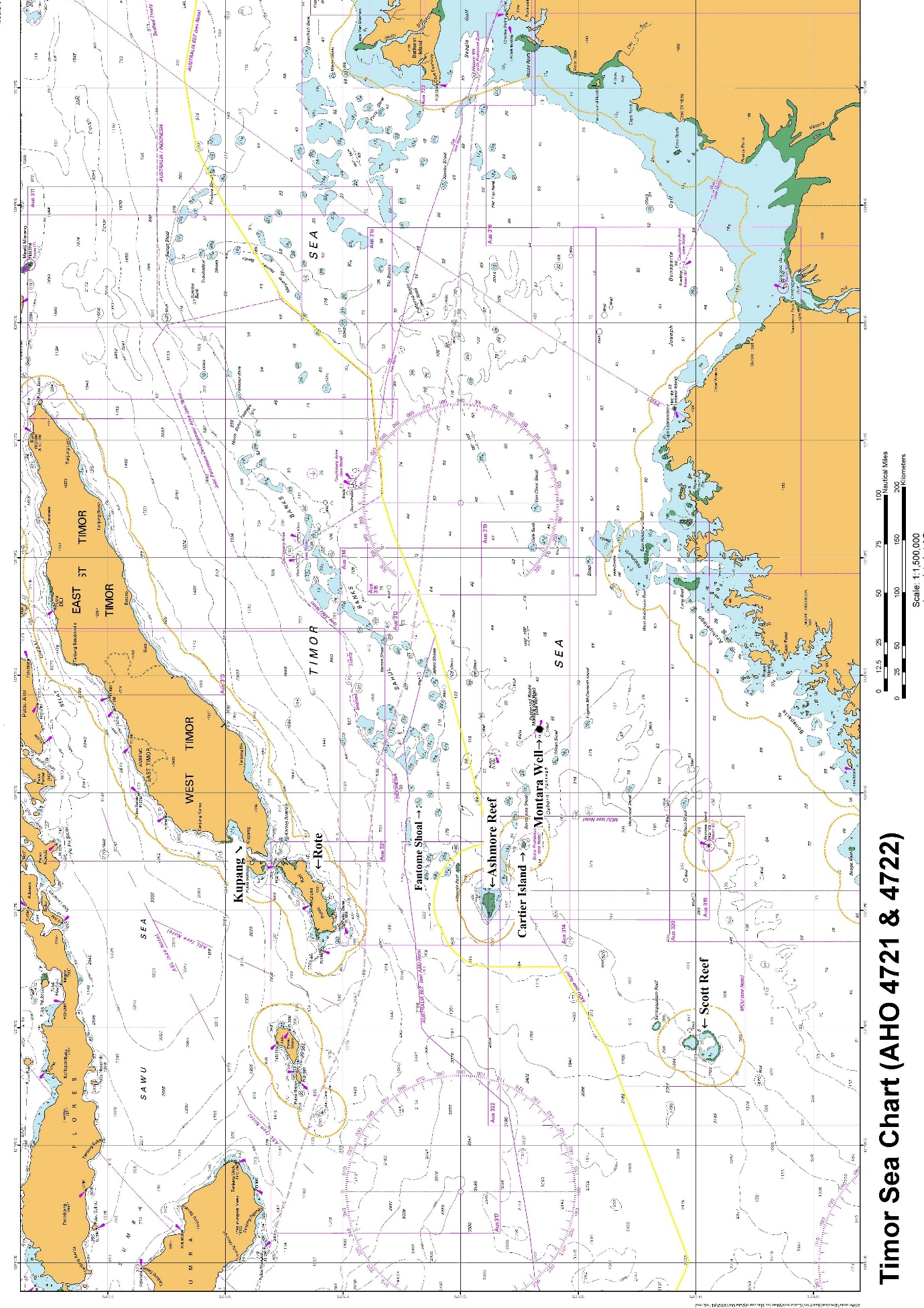
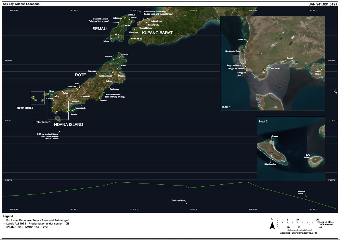
Name of witness | Daniel Aristabulus Sanda |
Affidavit details | Sworn on 18 August 2018; Bahasa version MFI 2. |
Transcript | XN: T122-157; XXN: T123-225; RXN: T225-228 |
Location of village | Oenggaut, near the south west extent of Pulau Rote
|
Oil timing | Between the middle to late September 2009. |
Nature of observations | The witness said his seaweed started to die, and he witnessed oil and fish dying (including big and small fish such as pilana and tuna). After two or three days, the seaweed turned white and after four days, the seaweed had died. The witness saw ‘blocks’ (of oil) which were of a yellow-ish and grey-ish colour, around the size of the circle made by his forefinger and thumb. They were attached to the witness’ ropes and seaweeds. This substance made his skin smooth and slippery ‘with oil’ to the touch. The water was dark and opaque. The witness also observed ‘colours like a rainbow’ on the surface of the water and smelt oil. |
Effect on seaweed farming | Mr Sanda attempted to replant using ‘seeds’ (being small pieces of fresh new branches; seaweed variety: sakol) purchased from Oeseli in March 2010, but those seeds died after a week. The witness has since been able to plant and harvest sakol seaweed. Before 2009, the witness was able to plant seaweed called cottonii hijau, which was tighter and thicker and heavier than sakol. The witness was not able to grow cottonii after 2010 because none was available. The witness did not see his neighbours growing cottonii. He did not know if other seaweed farmers on Rote grew cottonii after 2009. The witness made the following observations about growth before and after 2009. |
2002-2005 (inclusive): The seaweed looked healthy and grew well. The witness had three plots which had good, reliable yields and caused him to desire to increase his rope numbers. At the end of 2005, he was setting up a fourth plot. Towards the end of 2010: the witness was able to grow seaweed on 17 ropes, but did not harvest it. The growth was slow and the seaweed was soft and became white. | |
2011: 80 ropes. The growth was better, but the quality was not good (the seaweed was soft and whitish in colour and easily breakable). In 2010 and 2011, the sakol was soft and mushy and resulted in a lower portion of dry seaweed than the cottonii before and the sakol today. 2012: 160 ropes. The witness also noted that he was unable to produce as much wet seaweed from a single rope in 2012 as in 2008 and 2009. In 2008 a long rope could produce five baskets, and in 2012 it would only yield two baskets because the environment was not as healthy and therefore the seaweed was much smaller and not as good. 2013: 200 ropes. The production was still less per rope than in 2008-2009 (two or three baskets per rope) and of poorer quality (‘not big enough in comparison to previous years’). 2014: 227 ropes. Again, the production was not as good as in 2008-2009, producing two to three baskets and with smaller stems. 2015 – present: 227 ropes. Crops are growing and there are regular harvests. The growth is still the same and unhealthy, and crops have failed to thrive. The problems include small clump sizes, slower growth and lower dry to wet ratio seaweed weights. There has been no improvement in the health of the crops since 2015. Some of this evidence was questioned by Mr Scerri, who directed the witness to the notes of the sign-up meeting which recorded that, for example, in 2010 and 2011 the seaweed crop grown in that village was cottonii (T182:45-T183:06). There is also some discrepancy in the documents as to production figures (e.g. 10,500 kg in 2008 as reported in the Schedule to the Further Amended Statement of Claim as opposed to 18,000 kg in the sign- up meeting form: T199:42-T200:04). The witness said that 18,000 was the true figure in his mind. Mr Scerri also cross-examined on the influence of ‘ice-ice’ (a condition which turned seaweed white). However, in his affidavit the witness draws a distinction between the effect of ‘ice-ice’ and oil (at [108]).
|
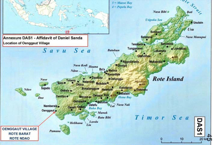
Name of witness | Silwanus Aplugi |
Affidavit details | Sworn on 20 August 2018; Bahasa version MFI-3. |
Transcript | XN: T234-238; XXN: T238-302; RXN: T:302. |
Location of village | Anarae, in the northern part of Ndao.
|
Oil timing | Mid to late September 2009. |
Nature of observations | The witness deposed that the seaweed was damaged. It became soft and there were dead fish in the surrounding area. Corals had also been detached from the bottom and floated on the surface. After three or four days, the seaweed was not producing anymore and there were dead birds. In the water there were bubbles of oil and the colour was yellowish and chocolate. When the witness entered the water and touched it his arms and lower limbs felt itchy. The water was less clear than before there were bubbles of oil. The bubbles felt itchy and looked like the form of candles and liquid. |
Effect on seaweed farming | Between April and early September 2009, production was more than 4,000kg. The seaweed was healthy. The witness grew both red and green seaweed in 2009, and believed the red produced slightly better harvests per rope. In XXN he stated that he had 100 ropes in 2009, but the harvest failed (T295:45-T296:02). In XXN, the witness suggested he produced 11,000 kg of seaweed in 2008. Mr Arnott put a sign-up meeting document to him which recorded his production as 10,000 kg for that year (T265:25). The witness then suggested his production was larger than that and varied between 15-17,000 kg (T266:20-26). The witness said that in 2010 and 2011, after struggles to find seed, he tried to grow red seaweed that was similar to the type he had grown previously. It did not yield a harvest. In 2012, the witness tried to grow ‘original’ seaweed (a third type of red seaweed; a soft variety) but in his affidavit deposed that it did not work. In XXN he deposed that the seaweed grew fast and he had 100 ropes, and it was strong and healthy such that he was able to do two harvests by the end of November 2012, harvesting 1800 kg of dried seaweed (T297:03-05). He was able to sell this for a profit. In RXN, he clarified that this seaweed dried to be ‘lighter’ than the other varieties he had previously grown (0.5 kg for each 20 kg of wet seaweed) (T303:03-04). In his affidavit, the witness deposed that he has not successfully grown seaweed since 2009, although he did try once more in 2017. |
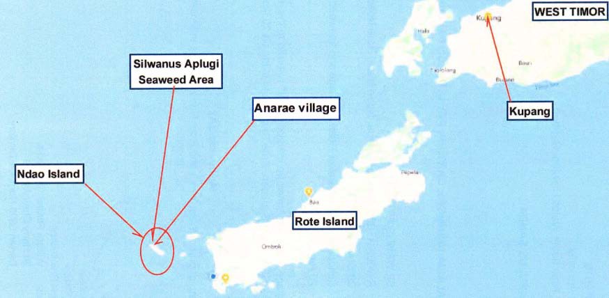
Name of witness | Adrian John Sibert |
Affidavit details | Sworn on 30 August 2018 |
Transcript | XN: T304-307; XXN: 307-329 |
Location of village | Sedeoen, Rote Barat Daya, Rote Island |
Oil timing | Late September 2009 |
Nature of observations | This evidence is largely proving up the sample Mr Sibert took of the affected water. The witness described white/off-white foamy patches floating on the top of the water which were between 30-50 square metres in diameter. There were dead fish (mackerel, bonito and smaller ‘pilchard’/’piladies’ bait fish) in these patches. The foam was around 100mm thick, the texture of detergent bubbles and had a crimson- y, detergent-y glow. The foam was distinct to surf wave foam, as it didn’t break up or dissolve and was denser. There were also mustard-coloured globular-looking things about half the size of a golf ball floating on the water, which slid between his fingers and fell apart when touched/squashed. The foam and globules went at least from the shoreline (where globules had washed up) out to 300m from shore. There were also foam patches at the ‘bombora’ reef the witness motored out to around 1.5km from shore. A few days later, the globules were still there along the beach where they had been washed up at high tide (in the harbour between Sedeoen and Nemberala). The witness also observed foam and globules along the Nemberala shoreline and in the lagoon, about 1km away from the shoreline. The foam and globules were visible for around 3 days. The witness described that the foam was in and around the ropes of seaweed on the beach near where he lives, and over the next few days or so the tips of the seaweed were turning white. If you touched the seaweed, it would turn to mush and had no strength to it. Over the next few weeks, the seaweed went white and broke off, the main part (‘trunk’) of the seaweed went droopy and appeared to be drying up, and the seaweed broke off the ropes. There was a lot less seaweed. |
Effect on seaweed farming | The dieback and death of the seaweed was evident in the month after the oil spill. The farmers tried to replant their ropes by breaking pieces from surviving plants and reattaching them, but without the success of the previous crops. In around December 2009, the witness observed that the seaweed crops in Sedeoen were struggling to survive with only around 30% visible on the ropes compared to what had been visible prior to the oil spill. Upon his return in 2012, the witness observed that the crops had not recovered and were still at around 30% of what had been visible prior to the oil spill. |
Name of witness | Gabriel Mboeik II |
Affidavit details | Sworn on 25 July 2018; Bahasa versions MFI-5, MFI-7. |
Transcript | XN: T330-335; XXN: T335-375. |
Location of village | Oelua, Rote Barat Laut, northwest Rote
|
Oil timing | September 2009 (although possibly August, as in XXN the witness deposed he did not visit his crops in August 2009: T367:31-35). |
Nature of observations | On the first day the witness noticed the oil, he noticed that the sea was full of colours. The ropes of seaweed had turned yellowish in colour and the seaweed was chocolate in colour. The smell of the seaweed was like solid oil. The seaweed felt soft to the touch and made the witness’ skin itchy. The seaweed had never looked/felt like that before. There were also small fish dead in the water, and where there were trees, there were blocks of oil attached to the trees. These things were observable for a month. In the following days, the seaweed died and washed away to the sea. |
Effect on seaweed farming | In 2006 and 2007 the witness experienced strong seaweed growth, but in 2007 there were hot temperatures around October/November and some seaweed broke and washed away. 2008 was the best year the witness experienced as a farmer. In January/February 2009, some seaweed broke off the ropes and washed away because of wind and waves, but then conditions returned to normal. The witness had been harvesting good yields of high quality seaweed just before the oil came. After September, there was no harvest at all. After the seaweed died, there was no seed to start a new crop. In 2010, the witness got enough red and green seaweed seed from Fisheries to seed two ropes, and grew 50 ropes of seaweed of 50m each. In 2010 the production was not good compared to 2008. The seaweed was small and could not grow bigger. In 2011, the growth was the same as 2010. There was not much seaweed to harvest compared to earlier years. The witness harvested on fewer days and only brought in small baskets. The dry weight was less than he had been used to in the good years. In 2012, the crop was gradually improving compared to 2011, but the problems of slow growth and branches breaking off continued. The harvest work was a little busier but the baskets were still small. In 2017, again the health of the seaweed crop improved a little, but the growth was slower, and yield was less, than before 2009. |
Name of witness | Gustaf Adolof Lay |
Affidavit details | Sworn on 23 August 2018; Bahasa version MFI-6, MFI-8 |
Transcript | XN: T376-380; XXN: T380-409; RXN: T409-411 |
Location of village | Tablolong, Kupang Barat, Timor Barat
|
Oil timing | Late September 2009. |
Nature of observations | The witness deposed that on the first day, the water changed colour: it was shiny, oily, and looked like a rainbow. There were blocks in the water that were colours like chocolate, greyish and yellowish. The seaweed had become limp. There were dead fish, animals and starfish in the sea. On the second day, the seaweed was worse. It was soft. The witness squeezed the blocks, which were as big as his fist. They were the texture of candle and oily, and made his hand itchy. On the fifth day, the witness took a boat out for the purpose of harvesting, but the crops were all destroyed. |
Effect on seaweed farming | In 2009 and earlier, the witness grew three types of cottonii seaweed (red, green and chocolate). The crop always looked healthy and strong. Between 2001 and 2009, the weather and water conditions made little difference to the growth and quality of the seaweed. The crops always grew well. In 2008, the witness produced 13,500 kg of dry seaweed. In 2009 it was less: 8,600 kg between February and September. Growth from February to early September 2009 was good. After September 2009, the seaweed did not recover and the witness did not harvest anything. There were no cottonii seeds to replant. In March 2010 the witness grew a different variety of seaweed, called sakol. The seed was from Semau Island, and did not look healthy and strong like the seaweed the witness grew previously; it had brown and white spots, but was at least alive. The growth was not good, and yielded only 900 kg of dried seaweed. In 2010, the witness deposed that only about 20 farmers in Tablolong managed to grow crops, and there was not enough seed for everyone. In 2011, the witness bought more sakol seed and produced 2,400 kg of seaweed. In 2012, the witness was able to produce 5,000 kg of seaweed. He attempted to add more ropes, but despite those attempts the growth of the sakol seed was not very good: slower growing and branches were turning white and breaking off. There were a number of small harvests. It was not as good as before the oil spill. In 2014, the sakol seaweed did not look like it would improve. It still had white branches and grew slowly. In 2015 the witness tried to start producing a new variety of seaweed, called SP. It grew faster and never looked sick, but its price was low. |
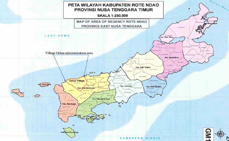
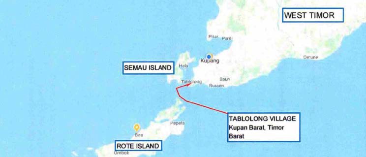
Name of witness | Semin Rachmat Polin |
Affidavit details | Sworn on 15 September 2016; Bahasa version MFI-10 |
Transcript | XN: T415-418; XXN: T419-438; RXN: T438 |
Location of village | RT/006, Desa Kuanheun, Kupang Barat (Map MFI-9)
|
Oil timing | Late September 2009. |
Nature of observations | The witness observed big (about 5m), medium and small (about 10cm) circles of oil on the surface of the water in his field of seaweed. The oil was many colours like a rainbow. After touching them, the witness’ body was oily and slippery. This lasted for 5-7 days. In the following days the seaweed detached from the ropes; died and washed away. The witness did not see anything else in the water. In Form V2 annexed to his affidavit, the witness deposed that there was oil on the surface of the water and the seaweed fell off the ropes. There was black on the ropes and the oil was as far as the eye could see. The oil lasted until December. |
Effect on seaweed farming | In 2008, the witness produced 1,600 kg of sakol seaweed. In 2009, the witness experienced good growth of sakol until the end of September. The seaweed became diseased and detached from the ropes. In 2010, the witness tried to produce seaweed but it did not grow. The witness did not grow seaweed in 2011. In Form V2 annexed to his affidavit, the witness deposed that the farmers at his village grew sakol seaweed. In 2007, the quality of the crop was good and it grew well. In 2008, the weather conditions were not quite as favourable: it was a late start but a very good crop. In March 2009, the quality of the crop looked good but failed miserably in September. In 2010, the seaweed was sick with white spots, and although the farmers tried to grow it, it failed. In 2011, the seaweed was still sick and of poor quality. In 2012, the seaweed was slightly better but still covered with white spots and breaking up; nothing like before 2009. In 2013, the seaweed was slowly improving but still sick with white spots. Some seaweed would stay on the ropes but would not grow. In 2014, there was a steady improvement but the seaweed was still growing slowly. |
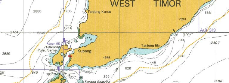
Name of witness | Johan P Lima |
Affidavit details | Sworn on 13 October 2016. |
Transcript | XN: T440-441. |
Location of village | 008, Regency Semau South, Kupang (Map MFI-11)
|
Oil timing | September 2009. |
Nature of observations | On the surface of the water there were thick blocks coloured grey-ish or black-ish and oily. If touched, it felt slippery and made the skin itchy. The seaweed was limp. |
Effect on seaweed farming | — |
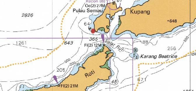
Name of witness | Dominggus Liman |
Affidavit details | Sworn on 17 October 2016. |
Transcript | XN: T442-445. |
Location of village | Neighbourhood 6/3, Akle Semau, Kupang Regency (Map MFI-12)
|
Oil timing | August/September 2009. |
Nature of observations | The oil looked like a rainbow and there were blocks that were black-ish or grey-ish in colour. They felt like oil. The seaweed became limp and detached. |
Effect on seaweed farming | Seaweed growth was good from January 2009 to August/September 2009. At that time, they detached. The witness had never seen that happen before. The seaweed did not recover in 2009. The witness tried to regrow seaweed in 2010 and it failed. |
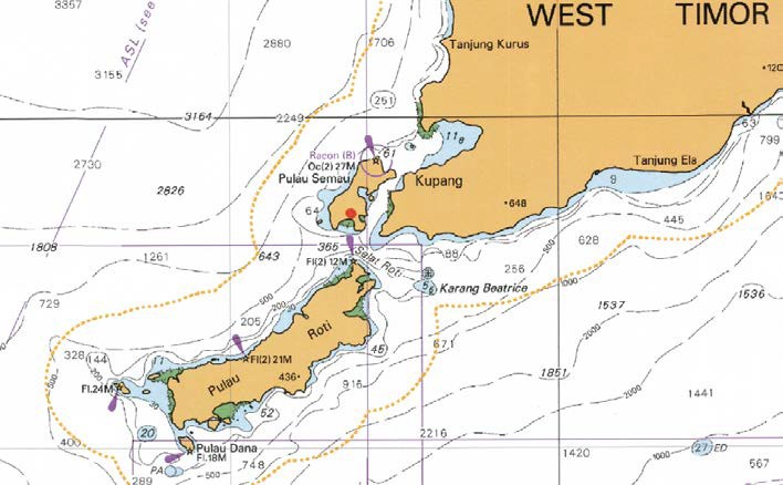
Name of witness | Zadrak Patolla-Ballo |
Affidavit details | Sworn on 26 September 2016. |
Transcript | XN: T450-453; XXN: T453-460. |
Location of village | Desa Letbaun RT 007/004, Semau, Kupang (MFI 13)
|
End of August 2009. | |
Nature of observations | There was oil, like kerosene on the surface of the ocean. There were lots of fish all dead along the beach. The oil smelt like lubricating oil, and very rotten. Many seaweed farmers got skin problems, and after eating the dead fish got irritated lips. The seaweed had oil all over it. It was about 500m away from the beach. When the witness tried to clean his seaweed by rubbing it, it fell off because it had turned light grey/white. It was soft to the touch. Over the next few days all the seaweed became mushy/sticky and fell off, broken off in little pieces and there were only a few big pieces left. |
Effect on seaweed farming | The witness had grown seaweed since 2002. The witness deposed that the type of seaweed grown was sakol, but in XXN agreed that it was cottonii (T459:24-26). In 2009, the seaweed was destroyed. It did not recover during 2009. In 2010, it was still damaged and the yield was very small in comparison to 2007 and 2008. In Form V2 annexed to his affidavit, the witness deposed that in 2007, the production and quality was ‘good’. In 2008, it was ‘extremely high’. In early 2009, it was good but the end of the year was very bad. In 2010, production was ‘low (half drop)’ and the quality was also bad. In 2011, production was ‘a bit low’ and the farmers attempted to grow sakol seaweed. In 2011, both sakol and cottonii varieties were grown. Sakol appeared to be more robust in poor conditions. |
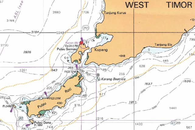
Name of witness | Abner Yopi Pallo |
Affidavit details | Sworn on 16 September 2016. |
Transcript | XN: T460-463; XXN: T463-465. |
Location of village | RT03, RW02, Batuinan, Semau, Kupang (MFI 14)
|
Oil timing | October 2009 |
Nature of observations | When the witness arrived at the beach, there was foam on top of the surface of the water. It shined like the colour of the rainbow. It smelt very rotten and felt shiny and slippery, and where it touched the skin it made it itchy. The seaweed was dirty with the foam which had stuck to the seaweed. On the second day, the seaweed seemed weak and after several days it became damaged and fell off the ropes. That had never happened before. The foam was still visible in 2010 by some villagers near Letbaun Village, but not in Batuinan. |
At the beginning of 2009, the witness’ seaweed and production was very good. In October 2009, it became weak and was destroyed. It did not recover in 2009. In Form V2 annexed to his affidavit, the witness deposed that seaweed farming began in the village in 2007, using cottonii. The seaweed thrived at that time, and increased in 2008. In early 2009 the quality and production was as excellent as 2008, but around September and October production decreased dramatically. In 2010, seaweed quality and production was extremely decreased. Harvests failed and the seaweed fell off the rope, falling off only 2-3 days after it was tied on. In 2011, the farmers began to grow sakol, but production did not increase. Seaweed production continued to decrease from year to year and has remained low. |
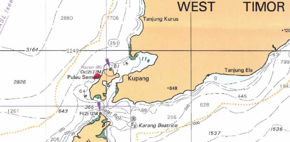
Name of witness | Petrus Ndolu |
Affidavit details | Sworn on 3 April 2017; Bahasa version MFI-17. |
Transcript | XN: T468-473; XXN: T473-484. |
Location of village | Baadale, Lobalain, Rote (seaweed farm in Nuse) (Map MFI-16)
|
Oil timing | October 2009 |
Nature of observations | The witness was at Nuse, where he farmed. The sea was the colour of a rainbow and there were dead fish floating on top of the ocean. There were chocolatey brown balls floating on top of the seaweed, which were oily to touch. The seaweed had wilted and gone yellow. It turned mushy and white in colour. The witness picked up his seaweed and tried to clean it, and his hands became oily. The seaweed stalks broke off. After the witness went home from the beach, his skin felt itchy. In November 2009 the witness boated to Baah, and the water on the way there was also the colour of a rainbow and there were balls floating on the water. In XXN, it was put to the witness that the timing of the oil was August 2009, and that Form V2 annexed to his affidavit did not record any observations of rainbow colours or brown balls in the water, instead setting out that the seaweed was ‘white, spotty and mushy’ and fell to the seabed when it was touched. |
Before the oil came, the seaweed growth in 2009 was very good. Between October and December 2009 the seaweed did not grow well any more. There was just a small harvest. In Form V2 annexed to his affidavit, the witness deposed that seaweed (both cottonii and sakol) was grown in Baadale from 2002. Cottonii was the preferred variety. There were usually four harvests each year. 2008 was the best year for Baadale in seaweed production. More cottonii was grown than sakol, but both crops were the healthiest they had ever been. The conditions were excellent and crops grew quickly. In 2009, there were two good harvests (May and July) but two were ruined (September and November). In 2010, the villagers attempted one harvest but the seed could not grow. The villagers stopped growing seaweed because of ‘bad production and quality’. |
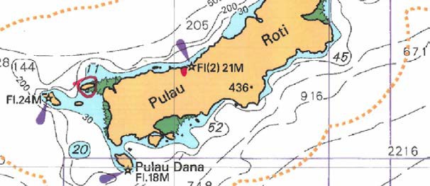
Name of witness | Abdul Rasyid Aitio |
Affidavit details | Sworn on 23 March 2017. |
Transcript | XN: T485-488; XXN: T488-492. |
Location of village | Papela, East Rote, Rote Ndao (farming also near Daiama village; about an hour from Papela by motorbike) |
Oil timing | End of September 2009. |
Nature of observations | The oil was brown and was like wax. It felt like oil and stuck to the witness’ hand. In the beginning, the seaweed felt okay because it had only just been covered in oil. Afterwards, it was soft or mushy. At Daiama, there were circular clumps of oil (of varying sizes, some less than a metre across, some as big as a table or cars; four or five metres across) floating in the water and when the sun shone on it, it looked like a rainbow. The seaweed was soft there and there were white bits on the end/white spots. It dropped from the ropes. The witness had never seen anything like that in the water before. |
Effect on seaweed farming | The witness began seaweed farming in 2000, near Papela and also near Daiama. In the beginning of 2009, the seaweed grew well. By the end of 2009, it was not good anymore, because there was oil that stuck to the seaweed. The seaweed did not recover in 2009. The witness did not grow seaweed in 2010, because it did not grow anymore. The witness’ child also grew seaweed and his plot had the same problem as the witness’ plot. |
Name of witness | Mica Erwin Johanis Penna |
Affidavit details | Sworn on 23 March 2017; Bahasa version MFI-19. |
Transcript | XN: T492-496; XXN: T496-510. |
Location of village | Matasio, RT07, RW04, Matili dusun, Rote Ndao. Seaweed farm located near Sotimori (about 30km away) (Map MFI-18)
|
Oil timing | September 2009. |
Nature of observations | The witness went to the beach and saw oil spilt about his seaweed. There was something in the water and on the shore that looked like light brown waxy grease. He could smell oil very strongly and the seaweed was covered in oil. The seaweed became mushy and soft and changed colour (to a pale colour) and then it died. When the witness cleaned his seaweed, the surface of the water looked like a rainbow. When he touched the seaweed, his hand felt oily and later it was itchy. The oil was everywhere, and it was in clumps as big as a fist. The sea felt like it was covered in oil and was a light brown colour. On the surface, there was wild seaweed that had died and small fish (as big as a finger) that were dead. At low tide, the coral and the rocks felt oily. This had never happened before. |
Effect on seaweed farming | The witness began seaweed farming in 2007. At the beginning of 2009, the seaweed was good. At the end the growth was not good. The seaweed did not recover in 2009. In 2010, the villagers planted new seedlings but they did not grow. The witness himself did not plant anything new, but had been told by others that their crops did not grow. |
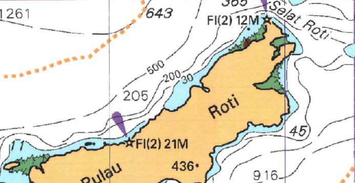
Name of witness | Taftinus Taek |
Affidavit details | Sworn on 22 March 2017. |
Transcript | XN: T511-513; XXN: T513-518; RXN: T518. |
Location of village | Dodaek village, Rote (Map MFI-20)
|
Oil timing | September 2009. |
Nature of observations | The witness saw clumps of wax that were brown in colour near the location of his seaweed (approx. 30m from the beach). The next day, there was also the smell of kerosene and there were clumps stuck to the seaweed. Not long after, the seaweed became weak and mushy and yellow and after about a week it died. The witness also saw dead fish and squid. |
Effect on seaweed farming | The witness began seaweed farming in 2002. From January to June 2009, the seaweed had good growth. In September it died. It did not recover in 2009. In 2010, the witness planted seaweed, but the yield was not as maximal as in 2008. In Form V2 annexed to his affidavit, the witness deposed that the Dodaek villagers farmed sakol seaweed and there were typically three harvests: April, September and at the end of the year, and seed for the new year would be collected in June. 2008 was the ‘golden year’ of seaweed farming. In 2009, there was only a successful harvest in April. There was normal growth until September. The farmers tried to dry their ropes, but it did not work. In 2010, the production and quality of the seaweed was still very poor. The farmers cleaned their ropes but the disease remained. In 2011, the conditions were the same but the farmers continued to grow seaweed. In 2011 and 2012 there was an increase in production but it was still nowhere near as good as 2008. |
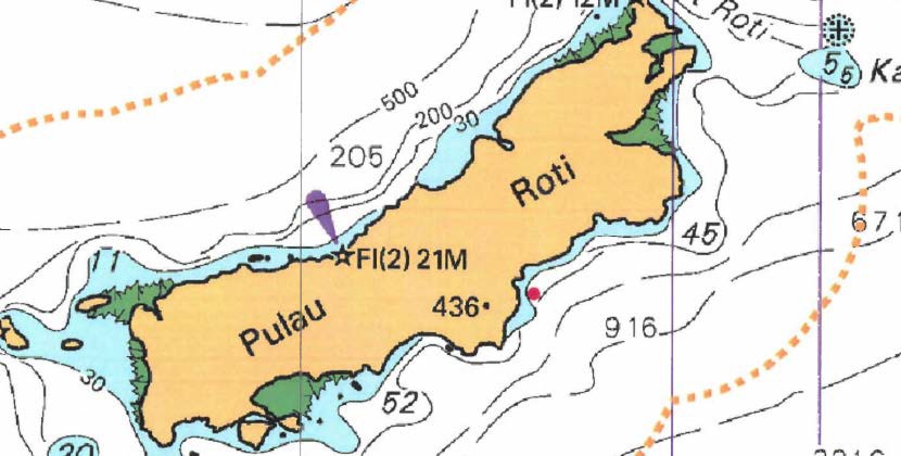
Name of witness | Semuel Messakh |
Affidavit details | Sworn on 9 February 2017. |
Transcript | XN: T518-520; XXN: T520-532; T533-534; RXN: T532-533. |
Location of village | Landu (small island off Rote Ndau) (Map MFI-21).
|
Oil timing | September 2009. |
Nature of observations | The witness saw oil on the surface, and a red colour and a blue colour, and it was on the sand. When it was close, it stuck to his hands and feet. Other seaweed farmers said that it made their skin itchy. There was oil on the mangroves and it smelt like diesel fuel. There were some dead dolphins on the seashore. The seaweed was damaged, with white spots. It fell off the ropes and was carried away by the current. This had never happened before. In Form V2 annexed to his affidavit, the witness deposed that Landu villagers saw the seaweed turn white and become soft. Some had a red covering on it, and the seaweed stopped growing and fell from the ropes. |
Effect on seaweed farming | The seaweed was damaged in September 2009 but growth was good before then in 2009. The seaweed did not get better in 2009. The witness did not grow seaweed in 2010. In Form V2 annexed to his affidavit, the witness deposed that Landu people started farming seaweed (cottonii) in 2002. In 2008, the seaweed grew well and there were 5-6 harvests. In 2009, seaweed did not grow well; there were only 3 successful harvests and production declined around September. 2010 was a bad year to grow seaweed. The harvest was not the same as 2007/2008. Farmers tried scraping and drying their ropes, but the result was the same. In 2011, many farmers gave up planting seaweed. In 2012, the farmers started growing sakol, which grew better than cottonii (although some of it still turned white). The production was higher than in 2011. |
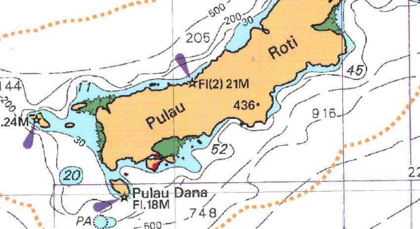
Name of witness | Yardin Adoni Lari Aplugi |
Affidavit details | Sworn on 5 April 2017. |
Transcript | XN: T535-537; XXN: T537-549. |
Location of village | Anarae, Ndao, Nuse, Rote (Map MFI-22).
|
Oil timing | September/October 2009. |
Nature of observations | There was a clump on top of the water. It felt like oil. On the first day, the seaweed was still good and fresh. That changed on the second and third days: the seaweed had sediment stuck to it and spots on it, and became damaged. It felt like oil to the touch. From the fourth day onwards, it became white and mushy and came off the ropes. This had never been seen before. |
Effect on seaweed farming | The witness began seaweed farming in 1997 (although in XXN he conceded that it is possible that there was no seaweed farming until 2005 and his memory was imprecise and vague). At the beginning of 2009, his seaweed was very good but in September/October it became damaged. The seaweed did not recover in 2009. The farmers tried to grow seaweed again in 2010 but it did not grow. |
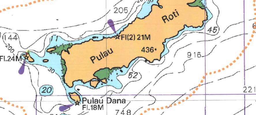
Name of witness | Nikodemus Ndun |
Affidavit details | Sworn on 12 October 2017. |
Transcript | XN: T557-560; XXN: T560-569 |
Location of village | Nemberala (buys seaweed from Nemberala, Sedeoen, Oelolot, dusun Aduoen, Boni and sometimes Oeseli and Boa)
|
Oil timing | — |
Nature of observations | — |
Effect on seaweed farming | In 2008, the witness was able to buy approximately six to seven trucks of seaweed each month, but the highest month was ten trucks (each truck being 6,000-8,000 kg when full). In January 2009, the witness was able to buy approximately six trucks of seaweed. In June 2009, the witness was able to buy approximately five to six trucks of seaweed. At the end of 2009, there was only one truck or a bit more of seaweed available to buy. In 2010, there was only approximately 4,000-5,000 kg of seaweed available to buy each month. It was difficult to buy seaweed and it was poor quality. It had many soft and white pieces when it was harvested and the branches were broken and small. 2010 was the worst year the witness had had for seaweed trading. |
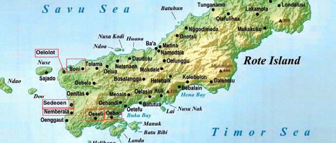
Name of witness | Lot Martinus Heu |
Affidavit details | Sworn on 12 October 2017. |
Transcript | XN: T570-572; XXN: T572-575. |
Location of village | RT5, RT4, Nemberala (farms at Nemberala and buys seaweed from Oeseli, Oenggaut and Oelolot)
|
Oil timing | September 2009. |
Nature of observations | — |
Effect on seaweed farming | Before the oil, the seaweed grew well. It stopped growing when the oil came in 2009 and did not recover. In 2010, the witness did not grow seaweed again. After the oil came in 2009, the witness was unable to find seaweed farmers with seaweed to sell to him. In 2010, the witness was only able to find a little seaweed to buy. The witness deposes in his affidavit that he became a seaweed farmer (cottonii) in 1999 and expanded his farms up until 2007. He stopped farming in 2009 after the oil arrived and the seaweed stopped growing and it was hard to find seed. He saw that other farmers’ crops were growing poorly. 2008 was the best year for growing seaweed. He also deposed that the seaweed had been very bad in 2010. He began as a trader in 2011 and business was slow because the crops were still struggling. It was difficult to buy much seaweed but better than in 2010 (it took about a month to fill a truck). The volume picked up a little more in 2012 (one truck per month quite regularly), and 2013 was better again (four or five trucks per month). 2014 was a good year (two truckloads every week and often more). In 2015, it was difficult to buy because other traders were offering better prices (around five truckloads per month). In 2017 the witness was able to sell around two truckloads per month. |
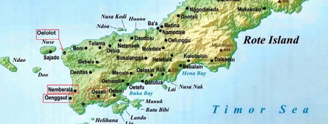
Name of witness | Thomas Dethan |
Affidavit details | Sworn on 5 April 2017. |
Transcript | — |
Location of village | Nuse, Ndao Nuse, Rote Ndao. |
Oil timing | Around October 2009. |
Nature of observations | There was a layer of oil slick in the water near the witness’ seaweed plot. When the morning light hit it and the sea was calm it had a rainbow colour on it. The witness had never seen it in the water. There were many small to medium sized dead fish, sea cucumber and sea urchins washed ashore on the beach and some in the water. The top of the witness’ seaweed turned white and started to break apart and feel mushy. It could fall off easily when waves hit it. Only the stem was attached to the ropes when they were taken away. The farmers tried to grow seaweed again but it did not grow. |
Effect on seaweed farming | — |
Name of witness | Resa Rehans Fatu |
Affidavit details | Sworn on 5 April 2017. |
Transcript | — |
Location of village | Mbalilendeki, Ndao Nuse, Rote Ndau. |
Oil timing | Around the end of 2009. |
Nature of observations | There was yellow oil on the sea surface. It looked like a rainbow when exposed by the sun. It formed in clumps and spread around the seaweed plots. It smelt like oil. When it contacted the seaweed, the seaweed turned spotty and white, then mushy and fell off the ropes. There were dead fish floating on the surface of the ocean and washed onshore. When the seaweed farmers came from the water they were itchy and developed a rash. |
Effect on seaweed farming | — |
Name of witness | Yermias Manafe |
Affidavit details | Sworn on 20 March 2017. |
Transcript | — |
Location of village | Sonimanu, Pantai Baru, Rote |
Oil timing | 2009. (Maybe September to October – after Indonesian Independence Day). |
Nature of observations | The oil came into the waters in Sonimanu’s seaweed area near Pukuafu. The seawater had a rainbow colour and there were dead fish around the sea shore. It was apparent that it affected the seaweed. All the seaweed became soft and its colour turned pale and white. It took less than a week for the seaweed to fall onto the seabed after the witness saw the oil. |
Effect on seaweed farming | — |
Name of witness | Anton Frans Alfonsus Matasina |
Sworn on 8 March 2017. | |
Transcript | — |
Location of village | Lifuleo, Landuleko, Rote Ndau |
Oil timing | Around the end of 2009. (September 2009). |
Nature of observations | Oil came into the waters near Lifuleo and the water around the witness’ seaweed plot turned reddish in colour. There were many dead fish in the water and washed up on the shore. The water smelt like kerosene. The witness had 45 ropes of seaweed ready to harvest but it all fell off to the seabed. It was soft with white spots. The witness thought it was a disease but had never seen anything like it before. All the crops died and washed away. The witness had itchy skin with a rash after going into the water. |
Effect on seaweed farming | — |
Name of witness | Watson Sodi Mbuik |
Affidavit details | Sworn on 17 February 2017. |
Transcript | — |
Location of village | Kolobolon, Lobalain, Rote |
Oil timing | Around October 2009. |
Nature of observations | The sea surface became oily and had rainbow colour. In the short time after, the seaweed became worse and had white spots on it. It was soft and white and fell easily to the seabed. All the crops died. The seaweed harvested later was sick and of poor quality. |
Effect on seaweed farming | — |
Name of witness | Marselinus Mesah |
Affidavit details | Sworn on 3 April 2017. |
Transcript | — |
Location of village | Oenggae, Pantai Baru, Rote |
Oil timing | Late 2009 |
Nature of observations | Many farmers complained their seaweed was dying on the ropes. There was something strange on the sea surface particularly in the morning and sunset time. The seawater looked oily and shining and its colour turned milky brown. There were dead fish on the sea shore. The seaweed became white and mushy like porridge. The crops died and washed away in the tides. |
Effect on seaweed farming | — |
Name of witness | Melkianus Mola |
Affidavit details | Sworn on 20 March 2017. |
Transcript | — |
Location of village | Oebau, Pantai Baru, Rote |
Oil timing | Around October 2009. |
Nature of observations | The oil came into the waters near Oebau’s seaweed farming area near Pukuafu in 2009. The sea surface looked different: it had shiny and rainbow colours on it. Not long after, the witness’ seaweed turned soft and easily fell off the ropes and washed away. There were dead fish floating in the water and some washed ashore. The witness got itchy skin and a rash after he went into the water. The oil stayed for around a month, maybe more. |
Effect on seaweed farming | The seaweed crop was good and healthy before the oil arrived, but it died in just a few days. |
Name of witness | Johan Mooy |
Affidavit details | Sworn on 2 April 2017. |
Transcript | — |
Location of village | Batutua, Rote Barat Daya, Rote Ndau |
Oil timing | 2009. |
Nature of observations | The oil came to water near Nusamanuk. There was foam on the sea surface, rainbow in colour. The clump of foam was part of a ‘sleek’ expanding many lengths. The sleek stayed for some time. There were dead fish on the seashore and the seaweed died. The seaweed turned pale, mushy and fell from the ropes. After farming in the deep sea, the witness’ skin felt itchy. |
Effect on seaweed farming | — |
Name of witness | Daud Nenokeba |
Affidavit details | Sworn on 26 September 2016. |
Transcript | — |
Location of village | Desa Uiasa, RT003/RW002, Kupang |
Oil timing | Around October 2009. |
Nature of observations | Oil came into the waters and the sea surface looked different. It had shiny colour and rainbow colours. The sea breeze smelled like diesel fuel. There were dead fish ashore in small amounts. The seaweed became sick and afterward it would not grow. |
Effect on seaweed farming | — |
Name of witness | Ogus Tananggau |
Affidavit details | Sworn on 23 March 2017. |
Transcript | — |
Location of village | Sotimori, Landau Leko, Rote Ndau |
Oil timing | September 2009. |
Nature of observations | A thin layer of oil was visible on the sea surface. There were rainbow colours in the sunlight. There was an orange waxy material on the beach. Fish and other sea creatures were found dead and washed up to shore. Within a week, the seaweed turned pale and mushy and washed off the ropes. It tasted oily and the witness was sick when he ate it. When the villagers ate the seaweed and fish, they got diarrhoea. Contact with the oil in the water made their skin itchy. |
Effect on seaweed farming | — |
Name of witness | Lorens Hendrik | ||
Affidavit details | Sworn on 26 September 2016. | ||
Transcript | — | ||
Desa Hansisi RT006/RW002, Semau, Kupang | |||
Oil timing | Around September/October 2009. | ||
Nature of observations | The witness saw something strange on the sea surface. It looked like waste from berthed ships – there were lumps in part, a little bit waxy with some black colour. When the current changed, it looked like leaked oil spread across the sea. There was something that smelled unusual. The witness was not sure if it was oil or not. Soon after, the seaweed went white and soft. It died and washed away and then became difficult to grow like it was sick. | ||
Effect on seaweed farming | — | ||
Name of witness | Axel Pierre Bruno Marcel Chalvet |
Affidavit details | Sworn on 21 August 2017. |
Transcript | XN: T580-584; XXN: T584-594; RXN: T594 |
Location of village | Boa, Rote Island
|
Oil timing | Sometime before the rainy season – around October/November 2009. |
Nature of observations | The witness observed that near his home there was a big mound of waxy, white, greasy substance floating all over the ocean. It looked like a very large river, of a width of a couple of hundred metres. It was moving with the wind. The white substance was accumulating in little whirlpools all over the beach on the sand, making clumps. It felt like greasy wax with salt/scales in it to the touch. The witness had not seen anything like it before. Over the next few days, that substance was coming and going, sometimes in big and sometimes lesser quantities. This continued for a couple of weeks. The witness sometimes went into the water during that time, and had to wash himself quite a bit when he did. The witness also described his observations about 7-10km south of Ndana Island, where he fished. There was lots of grease/wax floating around. His boat got really dirty. He also described his observations at Kite Beach (quite a bit of a waxy substance around there which accumulated on the beach) and Oenggaut Beach (pools of wax, but less on the beach and more in the water). The witness moors his boat in Oeseli harbour and usually it was difficult to get in and out because there was seaweed everywhere, but at the end of 2009 it was no longer difficult because there was no seaweed. During XXN, it was put to the witness that a contemporaneous document that described a white/yellow foamy substance (emails drafted by the witness’ mother) were more accurate than his recollection of a waxy/greasy substance but the witness rejected those assertions (T593:27-30). |
Effect on seaweed farming | — |
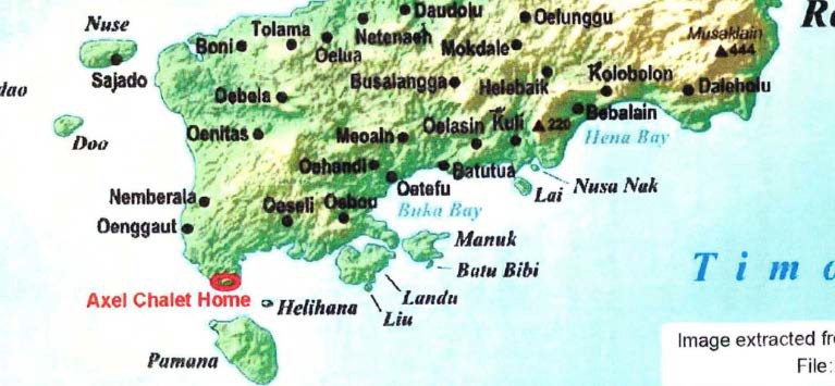
Name of witness | John Gregory Rogers |
Affidavit details | Sworn on 30 September 2017. |
Transcript | — |
Location of village | Nemberala, Rote |
Oil timing | October/November 2009. |
Nature of observations | There were brown masses floating on the surface of the sea. These masses were about four metres across. They were substantial enough to have collected debris from the water, including rubbish. The witness saw these masses on four or five separate occasions over a few weeks. The witness also observed a large dead fish (probably a groper) on one of these occasions, near Do’o Island. When kite boarding in October 2009, the witness noticed a black gummy substance sticking to his feet and his board. The black substance was almost everywhere along Kite Beach. It was difficult to get the substance off both skin and boards. The witness does not recollect seeing the substance on the sand, but experienced it almost every time he went into the water in 2010 and 2011. He does not recall it after 2011. |
Effect on seaweed farming | — |
Name of witness | John Douglas James Guiney |
Affidavit details | Sworn on 29 September 2017. |
Transcript | — |
Location of village | Nemberala, Rote
|
Oil timing | October 2009. |
Nature of observations | There was a significant level of pollution in the waters near Nemberala in 2009. In October 2009, the witness observed a black gummy substance sticking to his kite board equipment at Kite Beach. The substance was greasy and slippery. It was present at least until November 2009 (when the witness left Nemberala) and some of the substance was still observable when the witness returned in late April or May 2010. There was also a white foamy waxy substance on the logs and sticks at the beach, and on the seaweed ropes at Nemberala, with black waxy lumps mixed into it. When the witness lay on the sand, there were greasy oily marks on his clothes. There were also black greasy marks on his clothes after he went surfing. The witness deposed that he knew the substance was oil, because he had seen something similar in Wellington, NZ. |
Effect on seaweed farming | — |
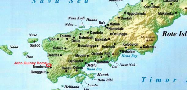
Name of witness | Bartolo La Macchia |
Affidavit details | Affirmed on 5 March 2019. |
Transcript | — |
Location of village | Kupang |
Oil timing | Late August/early September 2009. |
Nature of observations | The witness’ son observed something he thought was oil in the water 90nm SSE of Kupang (Fantome Shoals fishing area). The same oily substance was observed by the witness’ son 60-70nm east of Fantome (Mangola Shoals fishing area). All of the scampi and lobster the witness’ son fished in that area was ruined. 7-10 days later, the witness smelt oil in Tenau harbour and there was a sheen all over the water that stretched south and north to Kupang Bay. The witness was told other people had also seen oil in Kupang. |
Effect on seaweed farming | — |
Name of witness | Antony La Macchia |
Affidavit details | Sworn on 15 March 2009. |
Transcript | — |
Location | Kupang (the witness went fishing south east in the ocean and lived at Kelapa Lima) |
Oil timing | Late August/early September 2009. |
Nature of observations | There was a disturbance on the surface of the ocean at Fantome Shoal and rainbow colours on the water. It looked like diesel had been dropped onto the ocean. It was all around the witness’ boat on the water, spread as far as he could see. There was a strong smell of diesel. It was overpowering and gave the witness a headache. The fish catch in that area was contaminated. The fish were covered in a shiny substance that smelt strongly of oil. The catch could not be cleaned, because the water was dirty. A friend of the witness said he was travelling through oil in Australian waters, south of Ashmore reef, and had done so for 24 hours (subject to s 136 limitation). At Mangola Shoal, there was a smell of diesel and there was more oil at Mangola Shoal than Fantome Shoal. There were parts of the surface of the ocean that had the appearance of rainbow colours and there were puddles of thicker oil of a pale brown, muddy colour with pale brown lumps. Where the boat moved through the oil, it became creamy and foamy as if it had been mixed with milk. It made the witness think it formed an emulsion. Parts of the oil that did not become foamy were about 1cm thick on the surface of the ocean. The appearance of the oil in the water was not consistent – some it just looked dirty but it was clear something was not right/abnormal. After leaving the Mangola Shoal, the witness continued to see patches of brown oil and sheen. After steaming for 6-7 hours (about 100km) north-west to Kupang the witness saw clean water. The witness did not notice anything unusual at Kupang port. A week after the witness was fishing, he noticed the smell of oil near his home. He could see an oily sheen in streaks on the surface of the water in Tenau harbour. It was visible there at least a few days. Within a week or so of smelling the oil, the seaweed farms in the harbour were no longer there. They appeared to have ceased operating. |
Effect on seaweed farming | — |
Name of witness | Ghislaine Llewellyn |
Affidavit details | First affidavit sworn on 30 August 2018; Second affidavit sworn 28 March 2019. |
Transcript | — |
Location of village | — |
Oil timing | Survey undertaken 26-28 September 2009. |
Nature of observations | On the expedition boat on 27 September 2009, the witness observed a foul, strong, chemical smell in the air and felt a burning sensation at the back of her throat. There were patches and windrows of oil on the surface of the water. The characteristics varied in different areas. Samples of a waxy substance were collected. At times, there was a heavy blanket of oil on the surface of the water as far as the eye could see. It smelled like standing on the forecourt of a petrol station. The report annexed to the witness’ first affidavit provides detailed records of observations of the area around the oil spill and marine life encountered in the area. The witness’ second affidavit attaches a range of photographs. |
Effect on seaweed farming | — |
Name of witness | Simon Herbert Mustoe |
Affidavit details | Affirmed on 10 August 2018. |
Transcript | — |
Location of village | — |
Oil timing | Survey undertaken 26-28 September 2009. |
Nature of observations | The report annexed to the witness’ affidavit records the following observations (in addition to detailed information of the condition of the ocean and marine life). Oil sheen was encountered patchily and there were some concentrated lines of waxy particles. There was a pungent smell of oil which gave observers dry throats and a bad taste in the back of their mouths. Nearer the well head there was a thick layer of oil like a soft yellow crust accompanied by a moderately heavy oil sheen and a strong oil smell. Surface oil could readily be detected by extended patches of continuous glassy water, particles of white waxy residue and, in areas of moderate to high sheen thickness, the strong smell and presence of the soft yellow crust of unweathered wax with volatiles. Oil sheen was present for the majority of the three days of the survey. Oil sheen was found at distances beyond 70Nm from the well head. |
Effect on seaweed farming | — |
Name of witness | Matthew Smith |
Affidavit details | Affirmed 15 March 2019. |
Transcript | — |
Location of village | — |
Oil timing | Deployed as an aerial observer in September and October 2009. |
Nature of observations | One of the tasks of the witness was to identify the extremity of the oil and sheen. This was difficult because it did not form a clean unbroken line on the water surface. The oil and sheen was difficult to detect at times because it was variable in appearance. It was possible to detect water vessels’ tracks as they cut through sheen and waxy films on the water. Mud maps prepared by the witness reflect areas where observations of the oil were of: (a) a metallic/reflective substance; (b) orange/brown or yellow strings of substance in various concentrations; and (c) unconfirmed substance similar in appearance to brown/yellow strings. Very detailed reports of observations of sorties undertaken during September and October 2009 are annexed to the witness’ affidavit. |
Effect on seaweed farming | — |
Name of witness | James Watson |
Affidavit details | Sworn on 30 August 2018. |
Transcript | — |
Location of village | — |
Oil timing | Survey undertaken between 25 September 2009 and 4 October 2009. |
Nature of observations | 44% of transects surveyed were in waters visibly affected by oil. There was high biodiversity in the areas of the oil spill. Some dead/dying species were observed in affected waters, including a Common Noddy, a Horned Sea Snake and 17 adult birds. Response to the oil slick was species-specific. The oil was more prominent in transects north of the Montara oil well. Detailed observations of fauna are recorded the in the report annexed to the witness’ affidavit. |
Effect on seaweed farming | — |